

Backpropagation is a widely used approach to train complex neural nets in machine learning. It is an algorithm to compute the gradient of the cost (the deviation see Linear regression iterative) in each knot of the neural net. It does not optimize the net and it does not train it. It only computes the gradient for one data sample. That’s an important point to see.
When I first started to occupy myself with backpropagation, I read quite a few articles, looking for a useful description of this algorithm. But all I found where articles describing just the application of it. Some were talking about a chain rule for derivations to be used in the backpropagation, but I could not see any relation between the backpropagation, running from right to left in the neural net and a derivation which is directed from left to right.
So finally the idea came to me why not to try to deduce the maths for the backpropagation algorithm myself…. This article is the result of this idea

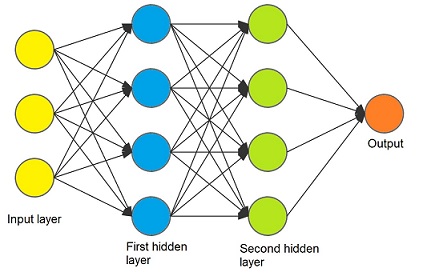
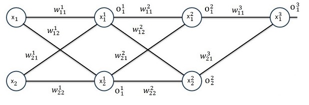
The neural net must have a certain form to be processed by the backpropagation algorithm. It consists of an input layer, hidden layers (the columns) and an output layer. One hidden layer contains a number of knots. Each knot must have the sum of all knots of the layer to the left multiplied by a given factor w for each input. Each knot has an activation function like the sigmoid function to be applied to compute its output.
So a neural net with 3 input features and 2 hidden layers looks like:
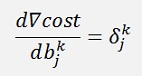
As it computes the gradient of the cost of the neural net, the math for it is based on this gradient and we have to calculate the gradient of the neural net get to the backpropagation.
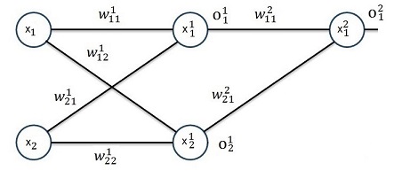
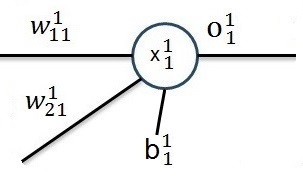
So I started with the simplest form of a neural net. It has just 1 layer, 2 input features and 1 output:
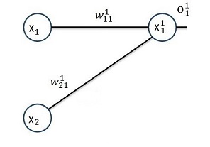
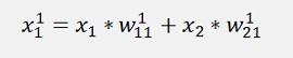
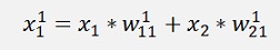
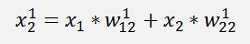
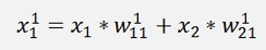
In this net we have the two inputs x1 and x2 (that correspond to one output y). Both are multiplied by a given factor w and added as:
Remark the indexing:

Is the element of the first layer and it leads from the row j to the row k. The elevated number is the index of the layer.
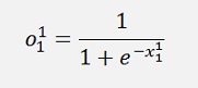
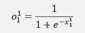
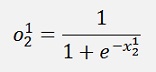
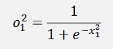
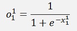
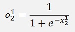
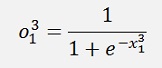
The result of this is fed into an activation function which is the sigmoid function here:
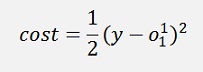
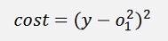
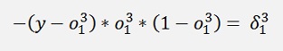
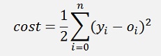
The cost is the square of the deviation of the approximated value from the given output y:
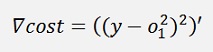
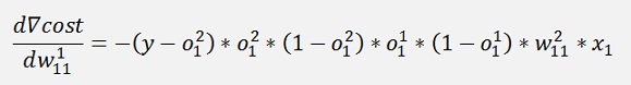
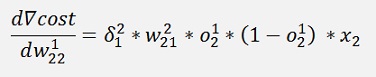
And the gradient of this with respect to w of that is:
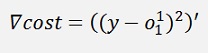
Where ∇cost is a vector with 2 rows here:
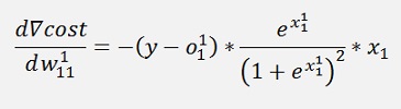
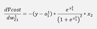
Now there is an interesting transformation:
The derivative of the sigmoid function is:
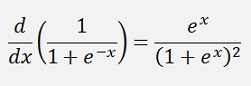
That can be written as
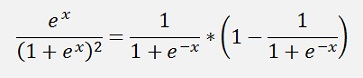
and with
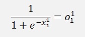
and therefore
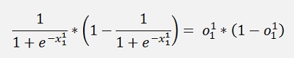
we can rewrite
That’s a cool step as o will be calculated later on and can just be reused like that. And here it is quite a simplification.
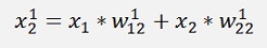
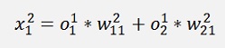
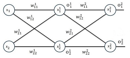
Now I did the same for a neural net with 2 layers with activation functions in each layer:
We start on the left side again:
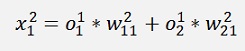
And the output:
The cost of this:
And the gradient of that:
With the same simplification as above:
If we have a closer look at the part
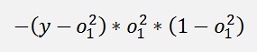
This part we got already further above in the net with one layer. It just had a lower layer index.
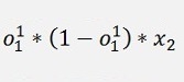
If we make the substitution
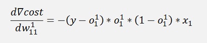
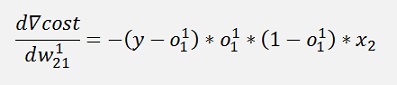
All gradients can be written as:
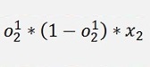
Without the input variable xk the gradient for w11 is the same as the one for w21 and the gradient for w12 is the same as the one for w22. That means we can compute a kind of a local gradient for the knot of x1 of the first layer and one for x2 of the same layer. For both we just have to multiply the local gradient of the knot to the right by the w factor that connects this knot to the actual knot and o * (1 – o).
And
is the local gradient of the knot to the right.
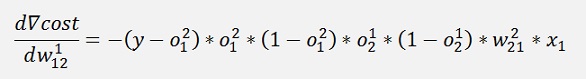
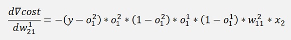
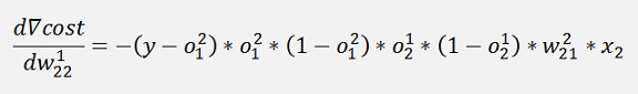
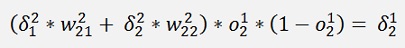
Now the same for 3 layers:
And again
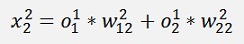
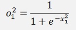
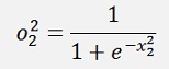
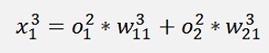
With all simplified same as above:
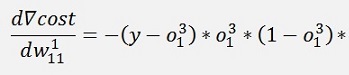
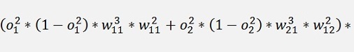
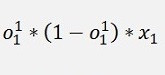
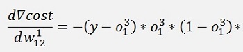
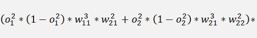
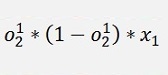
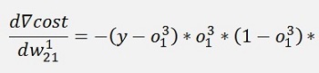
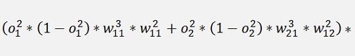
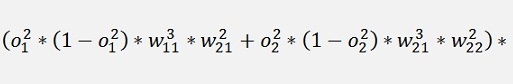
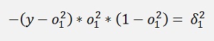
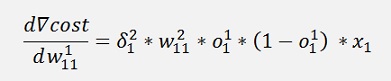
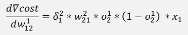
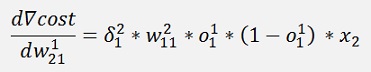
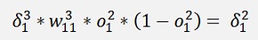
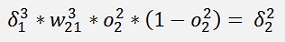
And again the local gradients
and additionally:
and with this:
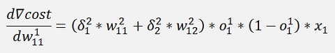
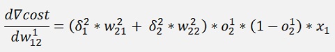
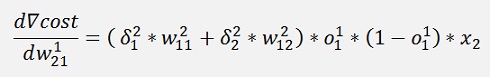
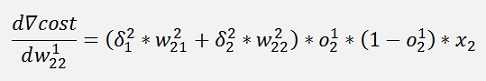
and
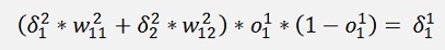
Are the local gradients for the first layer.
Again we can build a local gradient at the knot x1 and one at the knot x2 of the first layer. But now there are 2 local gradients on the right side. The both have to be multiplied by the connecting w factor added and the result is multiplied by o * (1 – o).
It can easily be seen that this is valid for more than 3 layers and more than 2 rows as well and it’s always the same: One local gradient is the sum of all gradients to the right multiplied by the connecting w-factor and the sum of that multiplied by o * (1 – o) of the actual knot.
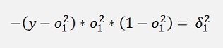
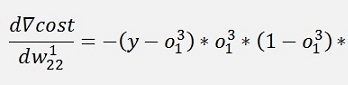
And indeed! The expression o * (1 – o) is the part of the chain of derivations (of the change rule) that can be related to the actual knot
And with
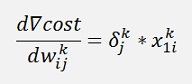
We have the factor to adjust the w-values.
That’s basically the process of backpropagation.
But that’s not all.
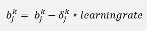
In my neural net there are some fixed offsets missing. A fixed offset like:
Can be treated like as a multiplication of w with fixed input 1 and so
One more step of complication is more than one output. There are applications were more than one output is required like.
And the backpropagation algorithm works better the more outputs are defined.More outputs affect the cost function which becomes a sum now.
And we get one local gradient for each output which affects only the calculation of the local gradients of the second last row.
Now it’s all for the backpropagation
To train a neural net the procedure is first to run from left to the right in the net and to compute all the x and o values in the net. This is done in a so called forward propagation. Then in the backpropagation the gradient for each knot of the net is computed. This must be done for each sample of the training dataset and for each local gradient the sum of these must be built and divided by the number of data samples (that means we have to store the sum of the adjustment for each w-value and for each offset in the net). That builds a mean gradient for each knot in the net and with this mean gradient each w-value and each offset is corrected like:
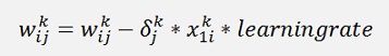
Then the procedure starts again and is repeated till all gradients become 0 and we are at the minimum of the cost.
But here the problems can start:
All the activation functions
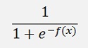
can add a local minimum to the approximating function where the backpropagation can get stock while searching for the global minimum. That makes the algorithm quite sensitive for a fine tuning. It’s not just feeding some data samples into it and it delivers the correct result. Backpropagation can require a special initialisation of the w-values and a variation of the activation functions like
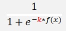
Varying k makes the activation steeper or flatter. That changes the behaviour of the algorithm quite badly.
The more knots the neural net has the more likely some work like this will be needed. But besides that the backpropagation is a very strong algorithm
To implement the algorithm we first have the build a useful structure for the data of the neural net. We need a structure to keep the w-values and offset for each knot, all the x- and o-values and additionally the local gradient and the sum of the delta for each w-value and for each offset.
I implemented a small class the represents one layer for that.
class TLayer
{
public int featuresIn;
public int featuresOut;
public double[] x;
public double[] o;
public double[,] w;
public double[] offs;
public double[] deltaOffs;
public double[] gradient;
public double[,] deltaW;
public function Act;
public function dAct;
Each layer gets a number of input features and a number of output features and two delegates to carry the activation function and its derivation (that gives me the possibility to change it or even to leave it and work without).
The definition for the delegate is:
public delegate double function(double value);
and the delegate functions are
public double Sigmoid(double x)
{
return 1.0 / (1.0 + Math.Exp(- 0.5 * x));
}
{
return 0.5 * x * (1 - x);
}
I assign them like
Act = Sigmoid;
dAct = dSigmoid;
In the constructor.
In the constructor of the class all member variables are initialised. The w-values I initialise to 0.5. Here comes another stumbling block: The activation function tends to saturate with very big or very small inputs. That means the w-values should not be initialised with too big or too small values.
These layers I keep in a list:
List<TLayer> net = new
List<TLayer>();
And assign them
tempRow = new TLayer(4, 2);
net.Add(tempRow);
tempRow = new TLayer(2, 2);
net.Add(tempRow);
For a neural net that has 4 input features, 2 layers and 2 outputs.
The forward propagation looks like:
private double[] ForwardProp(double[] x)
{
int i, j, k;
TLayer actLayer = net.ElementAt(0);
double[] actX = new double[x.Length];
for (i = 0; i < x.Length; i++)
actX[i] = x[i];
for (i = 0; i < layers; i++)
{
for (j = 0; j < actLayer.featuresOut; j++)
{
actLayer.x[j] = actLayer.offs[j];
for (k = 0; k < actLayer.featuresIn; k++)
{
actLayer.x[j] = actLayer.x[j] + actX[k] * actLayer.w[k, j];
}
actLayer.o[j] = actLayer.Act(actLayer.x[j]);
}
for (j = 0; j < actLayer.x.Length; j++)
actX[j] = actLayer.o[j];
if(i < layers - 1)
actLayer = net.ElementAt(i + 1);
}
return actLayer.o;
}
It gets the x-values of one data set, computes all x- and o-values in the net and returns an array of all outputs.
The backpropagation is a bit more complex
private void BackwardProp(double[] x, double[] y)
{
int i, j, k;
TLayer actLayer = net.ElementAt(layers - 2); // actual computed layer
TLayer layerRight = net.ElementAt(layers - 1); // nex layer to the right of the actual one
double[] actX = new double[x.Length];
for (j = 0; j < actLayer.x.Length; j++)
actX[j] = actLayer.x[j];
actLayer = net.ElementAt(layers - 1);
for (j = 0; j < actLayer.featuresOut; j++)
{
costSum = costSum + ((y[j] - actLayer.o[j]) * (y[j] - actLayer.o[j]));
actLayer.gradient[j] = (y[j] - actLayer.o[j]) * -actLayer.dAct(actLayer.o[j]);
}
for (j = 0; j < actLayer.featuresIn; j++)
{
for (k = 0; k < actLayer.featuresOut; k++)
{
actLayer.deltaW[j, k] = actLayer.deltaW[j, k] + actLayer.gradient[k] * actX[k];
}
}
for (j = 0; j < actLayer.featuresOut; j++)
{
actLayer.deltaOffs[j] = actLayer.deltaOffs[j] + actLayer.gradient[j];
}
if (layers > 1)
{
for (i = layers - 2; i >= 0; i--)
{
actLayer = net.ElementAt(i);
layerRight = net.ElementAt(i + 1);
if (i > 0)
{
TLayer layerLeft = net.ElementAt(i - 1);
for (j = 0; j < layerLeft.o.Length; j++)
actX[j] = layerLeft.o[j];
}
else
{
for (j = 0; j < x.Length; j++)
actX[j] = x[j];
}
for (j = 0; j < actLayer.featuresOut; j++)
{
actLayer.gradient[j] = 0;
for (k = 0; k < layerRight.featuresOut; k++)
{
actLayer.gradient[j] = actLayer.gradient[j] + (layerRight.gradient[k] * layerRight.w[j, k]);
}
actLayer.gradient[j] = actLayer.gradient[j] * actLayer.dAct(actLayer.o[j]);
actLayer.deltaOffs[j] = actLayer.deltaOffs[j] + actLayer.gradient[j];
for (k = 0; k < actLayer.featuresIn; k++)
{
actLayer.deltaW[k, j] = actLayer.deltaW[k, j] + actLayer.gradient[j] * actX[k];
}
}
}
}
}
It gets the x- and y-values of one data set and computes all local gradients and the sum of the delta-w and delta-offsets in the net.
With this the w-values and the offsets can be adjusted with:
private void UpdateValues()
{
int i, k, l;
TLayer actLayer = net.ElementAt(layers - 1);
for (i = 0; i < layers; i++)
{
actLayer = net.ElementAt(i);
for (k = 0; k < actLayer.featuresOut; k++)
{
for (l = 0; l < actLayer.featuresIn; l++)
{
actLayer.w[l, k] = actLayer.w[l, k] - actLayer.deltaW[l, k] / samples * learning_rate;
}
actLayer.offs[k] = actLayer.offs[k] - actLayer.deltaOffs[k] / samples * learning_rate;
}
}
}
The forward propagation and the backpropagation are run in a loop over all data samples and when this loop is done the update values function is called and the w- and offset-values adjusted. Then the procedure starts again until a maximum number of loops are done. Here I use a different approach from what I did in Gradient descend and Logistic Regression with the sigmoid function. There I checked change of the cost and quit the loop if this change is small enough. Here the cost can oscillate a bit because of local minimums that can be passed during computation and due to that the cost can become negative for a while. That’s why I do not check its change but run a big number of loops. That works quit fine
I implemented a sample project for the backpropagation and as I already used this data set in www.mosismath/LogisticRegression.html Logistic Regression with the sigmoid function it might be interesting to compare these 2 approaches
The Iris data set contains characteristic data of 150 Iris flowers and as I like flowers.
One data sample contains the following information:


I took the last 5 samples of each type to build a test data set. Same as I did it for the logistic regression. The rest of the 150 samples I use for training.
The data is held in separate class data and I read the samples from the csv file data.csv which is included in the project.
It would be possible to use the data the same way I did it in the logistic regression and to train one parameter set of w- and offset-values for one neural net with 2 layers, 2 rows and 1 output for one flower type. I did this and it worked fine for the Iris Setosa and the Iris Virginica. But the Iris-Versicolor got stock at a local minimum first. I had to change the initialisation of the w-values in the first layer to:
tempLayer = net.ElementAt(0); // initialisation for Iris-versicolor.csv"
tempLayer.w[0, 0] = -1.0;
tempLayer.w[0, 1] = 1.0;
tempLayer.w[1, 0] = -1.0;
tempLayer.w[1, 1] = 1.0;
to have the algorithm converging at the global minimum. Like this it worked fine.
But that’s not the best solution. The backpropagation works better if there is more than one output in the neural net. So I use 2 outputs. The flower type I number as
Iris-setosa = 1
Iris-versicolor = 2
Iris-virginica = 3
And this numbering I use binary to set the outputs for the neural net:
Iris-setosa => output 1 = 0 ; output 2 = 0
Iris-versicolor => output 1 = 1 ; output 2 = 0
Iris-virginica => output 1 = 1 ; output 2 = 1
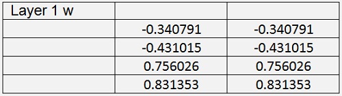
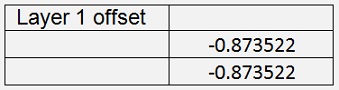
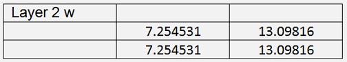
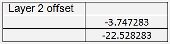
With this and 60000 iterations with learningrate = 0.4 the backpropagation algorithm computes the values:
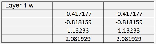
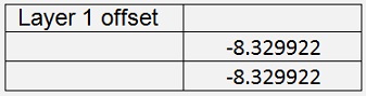
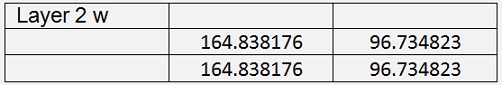
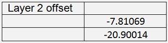
With
Cost = 0.01587
The test program detects all 15 flowers correct with quite high probability of 98.25 %. That’s cool and even works better than the logistic regression
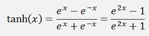
It is -1 for big negative values and 1 for big positive values and an interesting detail is: It saturates a bid slower than the sigmoid function. That makes it a bit less sensitive to get stock in saturated condition.
As the activation function should have an output range of 0 to 1 we cannot use the tangenshyperbolicus as is. The activation function using tanh should look like:
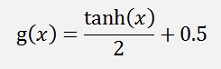
For the backpropagation we need the differentiation as well.
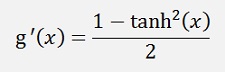
Implemented in the TLayer class that’s:
public double TanH(double x)
{
return Math.Tanh(x) / 2.0 + 0.5;
}
public double dTanH(double x)
{
return (1 - x * x) / 2;
}
As the tanh saturates slower than the sigmoid function, I had to reduce the learning rate to 0.2. With this and 60000 iterations I got:
With Cost = 0.0146
It works even a bit better than the sigmoid function.
The test program detects all 15 flowers correct with the same probability of 98.2 as did the algorithm using the sigmoid function.