

In machine learning there is quite often to situation that we want to recognise a certain pattern in a sequence of data or make decisions according to the evaluation of a set of data. That means we need to find function to a set of input vectors that can give an output of “yes” or “no”, “is” or “is not” or “good” or “bad” to each input vector. A numerical input should be converted to a digital output with of course as few wrong answers as possible. This is a minimizing algorithm somehow similar to the Gradient Descend . Only that the approximating function must yield a digital output.
This is achieved by using the Sigmoid function.
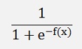
The Sigmoid function is given by:
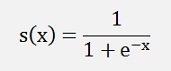
This Sigmoid function has an output like
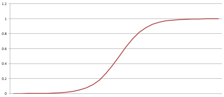
For big negative values of x it is 0 and for big positive values it becomes 1 and if it is applied to a function f(x)
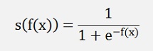
It converts the output of f(x) into a probability between 0 and 1.
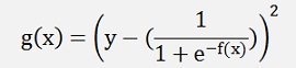
That means if we have a set of input data consisting of an input vector x1, x2,…,xn that has a digital output y, this can be approximated by a function
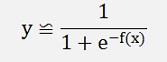
With y as the digital output and f(x) as a polynomial function like r1*x1 + r2*x2+...+ offset and x1..xn the input data to y.
And finding the best approximation means to find the minimum of this:
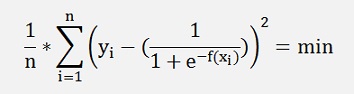
by the best setting of r1…rn and the offset.
And that is done by a Gradient Descend algorithm.
For the Gradient Descend we need to build the gradient for the above formulation.
This differentiation I inserted into the Gradient Descend algorithm I already implemented in Gradient Descend.
Now the only thing that remains to determine is f(x) and that depends on the data and the behaviour of its origin

In the web I found the Iris data set. This is a very nice data set containing characteristic data of 150 Iris flowers and as I like flowers, I use this data set to implement a logistic regression algorithm and build a small binary tree of it's result.
The Iris data set contains the following information in one row:
By the way:


To implement a logistic regression with this data first the function f(x) of
must be determined. As all 4 input values (sepal and petal length and width) do only fit to a certain plant if they are within a certain range the function f(x) must have a clear maximum somewhere. Therefore I use a second degree polynomial for eac input value:
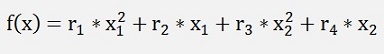
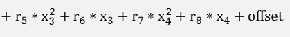
So we get double as much output variables as input.
For this function the differentiations for r1 to r8 must be built now. That’s not too difficult:
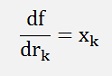
if k is even and
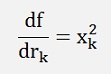
if k is odd.
With this and the application of the Chain rule the differentiation of the derivation for our Gradient Descend becomes
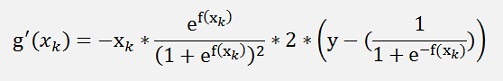
if k is even and
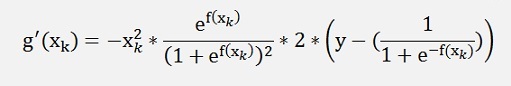
if k is odd. This formulation put in my Gradient Descend algorithm in the update_rise function becomes:
double[] update_rise(Collection<double[]> values, double[] rise, double learning_rate)
{
int i, j;
double[] d_rise = new double[features_out];
double[] x;
double y;
double e, e2;
double[] tempSum = new double[2];
double tempValue;
for (i = 0; i < features_in; i++)
{
d_rise[2 * i] = 0;
d_rise[2 * i + 1] = 0;
tempSum[0] = 0;
tempSum[1] = 0;
for (j = 0; j < samples; j++)
{
x = values.ElementAt(j);
y = x[features_in];
e = Math.Exp(F_x(x, rise, offset));
tempValue = 2.0 * x[i] * e / (1.0 + e) / (1.0 + e) * (y - 1.0 / (1.0 + 1/e));
tempSum[0] = tempSum[0] - x[i] * tempValue;
tempSum[1] = tempSum[1] - tempValue;
if (Math.Abs(tempSum[0]) > 1e6)
{
d_rise[2*i] = d_rise[2*i] + tempSum[0] / samples;
tempSum[0] = 0;
}
if (Math.Abs(tempSum[1]) > 1e6)
{
d_rise[2*i+1] = d_rise[2*i+1] + tempSum[1] / samples;
tempSum[1] = 0;
}
}
d_rise[2 * i] = d_rise[2 * i] + tempSum[0] / samples;
d_rise[2 * i+1] = d_rise[2 * i+1] + tempSum[1] / samples;
}
for (i = 0; i < features_out; i++)
{
rise[i] = rise[i] - learning_rate * d_rise[i];
}
return rise;
}
with
double F_x(double[] x, double[] rise, double offs)
{
int i;
double res = offs;
for (i = 0; i < features_out / 2; i++)
{
res = res + x[i] * x[i] * rise[2 * i] + x[i] * rise[2 * i + 1];
}
return res;
}
For the cost_function I had to modify the updata_values function like:
double[] update_values(Collection<double[]> values, double[] rise)
{
double[] predictions = new double[samples];
double[] x;
for (int i = 0; i < samples; i++)
{
predictions[i] = 0;
x = values[i];
predictions[i] = 1 / (1 + 1 / Math.Exp(F_x(x, rise, offset)));
}
return predictions;
}
With the Sigmoid function the Gradient Descend algorithm becomes a bit sensitive on too big changes and there is no more clear relation between the mean of the deviations and the offset in f(x). So I had to modify the update of the offset a little. In this implementation the offset is incremented by a fixed step in each iteration and if the algorithm overshoots, this step is divided by 2 and its sign is switched. So the update of the offset changes its direction and step. That should prevent from an next overshoot in the other direction and approach the minimum cost value.
With this the loop to find the minimum deviation looks like:
while ((Math.Abs(divCost) > 1.0e-8) && (count < 1000))
{
rise = find_min(data.values, rise, learning_rate, iterations);
divCost = oldCost - cost;
if (divCost < -1.0e-5)
{
step = -step / 2.0;
}
lastCost = oldCost;
oldCost = cost;
cost_history[count] = cost;
offset = offset - step;
count++;
}
with
double[] find_min(Collection<double[]> values, double[] rise, double learning_rate, int maxIers)
{
int count = 0;
double oldCost = 100000;
double divCost = oldCost - cost;
double[] ret = new double[2];
while (Math.Abs(divCost) > 1.0e-6 && count < maxIers)
{
rise = update_rise(values, rise, learning_rate);
cost = cost_function(values, rise);
divCost = oldCost - cost;
oldCost = cost;
count++;
}
return rise;
}
With this algorithm we have to find the approximation with minimum deviation once for each plant and will get a polynomial for f(x) for each plant. Therefore the data set must be prepared. I made 3 copies of the set and replaced the name of the plant in these copies as follows: In the data set for the Iris Setosa I replaced the name “Iris Setosa” by a 1 and the other names by a 0. For the other data sets I did the same for the other plants. Then I removed 5 samples of each plant from these data sets and took them for a “test data set”.
With the remaining data sets I got the following results:
Iris Versicolor
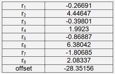
With a cost of 0.04352
Iris Setosa
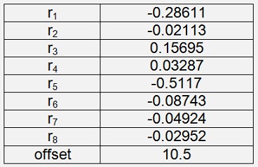
With a cost of 0.00046
Iris Virginica
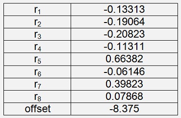
With a cost of 0.0116
That’s not too bad
With these results we can set up a small binary tree that recognizes the plant of each data sample in the test data set.
One knot of the tree consists of an approximating function f(x) and a triggering function, the Sigmoid function in this implementation, and the tree looks like:
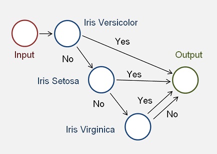
One such knot is a simple function that computes the probability that the input data belongs to one certain plant in the function.
double calc_probability(double[] x, double[] rise, double offset)
{
return 1 / (1 + 1 / Math.Exp(F_x(x, rise, offset)));
}
With the f(x) function
double F_x(double[] x, double[] rise, double offs)
{
int i;
double res = offs;
for (i = 0; i < features_out / 2; i++)
{
res = res + x[i] * x[i] * rise[2 * i] + x[i] * rise[2 * i + 1];
}
return res;
}
This function gets the sample data in the array x, the 8 rise values and the offset that fits to one plant and returns the probability that the input data sample fits to this plant. If this probability is bigger than 0.5, the input data belongs to this plant, if it is smaller than 0.5 it does not and the next plant must be tried. That makes 3 trials for our 3 plants and each trial is one neuron.
In code that’s
for (i = 0; i < samples; i++)
{
x = data.values.ElementAt(i);
probability = calc_probability(x, rise.ElementAt(0), offset[0]);
if (probability > 0.5)
{
flowerName = "Iris-versicolor";
}
else
{
probability = calc_probability(x, rise.ElementAt(1), offset[1]);
if (probability > 0.5)
{
flowerName = "Iris_setosa";
}
else
{
probability = calc_probability(x, rise.ElementAt(2), offset[2]);
if (probability > 0.5)
{
flowerName = "Iris_virginica";
}
else
{
flowerName = "Not recognized";
}
}
}
// output the result
}
With the 15 data samples as test data the application gets:
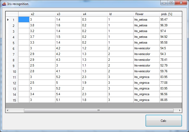
All 15 plants are recognised correct with a probability between 52.76 % and 96.56 %. O.k. that’s not too narrow. But with just 135 samples for training that’s quite o.k.
I implemented one application the LogisticRegression_Iris for the so called training. This application computes the rise and offset parameters. These parameters I use in the application NeuralNet_Iris to compute the test data.