

When the topic digital filters came to me I for a first time I asked myself: How is the bridge between an analogue filter with its transfer function in frequency domain and a digital filter with its broken rational function.
A digital filter is defined by its broken rational function in the z-domain.
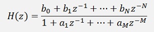
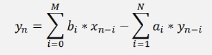
With the formulation for the online calculation:
Low pass filter
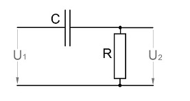
An analogue filter is usually defined by its transfer function in the frequency domain like for instance a simple low pass RC element:
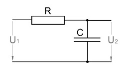
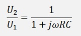
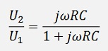
Has the transfer function:
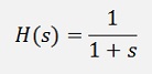
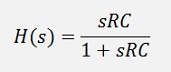
This RC element has a transfer function in the Laplace domain like:
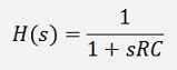
To get there we simply have to replace the jω by s. That’s it.
(To get the behaviour like inrush output this equation would have to be multiplied by the Laplace transformed unit step and the resulting equation would have to be transformed back into time domain. Just to be mentioned)
To get the formulation for the digital implementation of such a filter is a bit a different story. Therefore the transfer function in the Laplace domain must be transformed into the transfer function in the z domain. That sounds quite frightening: Huuu... z transformation
 . But
in fact it does not have too much to do with z transformations.
. But
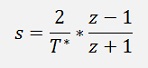
in fact it does not have too much to do with z transformations.There is just a substitution called bilinear transformation. It substitutes s like:
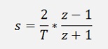
With T as the sampling time which is 1 / fs.
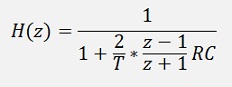
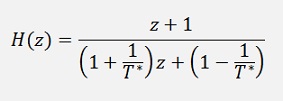
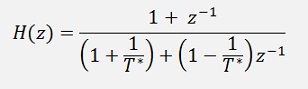
With this substitution the transfer function H(z) becomes
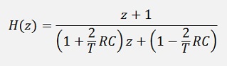
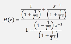
Or a bit rearranged
and as the cut off frequency is
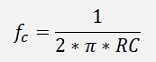
or
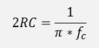
and

We can say
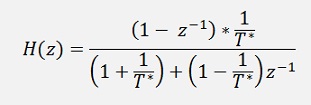
And our transfer function becomes
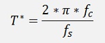
The value T* is quite an important value in digital filtering and we will meet it again with the other filters. It is the relation between sampling frequency and cut off frequency of a digital filter. So never forget that
In the literature they usually work with T*. But that’s not too clearly mentioned. In this case the transfer function in s would be:
and
Now. At the end we need a transfer function looking like:
So our transfer function must be divided by z2:
and

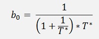
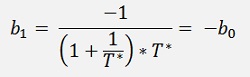
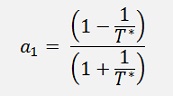
So we get:
and have our digital filter parameters

And the online calculation would be like:
The parameter a0 is not mentioned. It is mathematically on the left side of the equation.
This formulation means: I have an input signal y_in which can be a signal that is read new in each iteration or it can be a sequence of a signal in form of a list or array. For the processing I need the actual signal y_inn and the one of the las iteration y_inn-1. Additionally the output signal that has been computed in the last iteration y_outn-1 is needed. This signal and y_inn-1 must be stored from one iteration to next. If the input is a list, I can use the last index for y_inn-1 and just have to store y_outn-1. In my sample project I put the output signal into an array to and so I can use the last index of this output to.
To put that into code is not too complicate:
// Calculate T
t = 1.0 * Math.PI * fc / fs;
// Create an input singal
for (i = 0; i < datapoints; i++)
{
t_in[i] = i / fs;
y_in[i] = 20.0 * Math.Sin(2.0 * Math.PI * t_in[i] * f
}
// Build filter parameters
b[0] = 1 / (1.0 + 1.0 / t);
b[1] = b[0];
a[0] = 1.0;
a[1] = (1.0 - 1.0 / t ) / (1.0 + 1.0 / t );
// Process the singal and compute the output
y_out[0] = 0;
for (i = 1; i < datapoints; i++)
{
t_in[i] = i / fs;
y_out[i] = y_in[i] * b[0] + y_in[i-1] * b[1] - y_out[i-1] * a[1];
}
This short sequence builds a sample signal with the frequency f and a sample frequency fs and filters it with the cut off frequency fc. The variable datapoints is the number of samples and y_in, y_ou and t_in are arrays with the length datapoints.
O.k. it’s probably no too interesting to build a filter of just the first order. But it’s a good way to understand how things work.
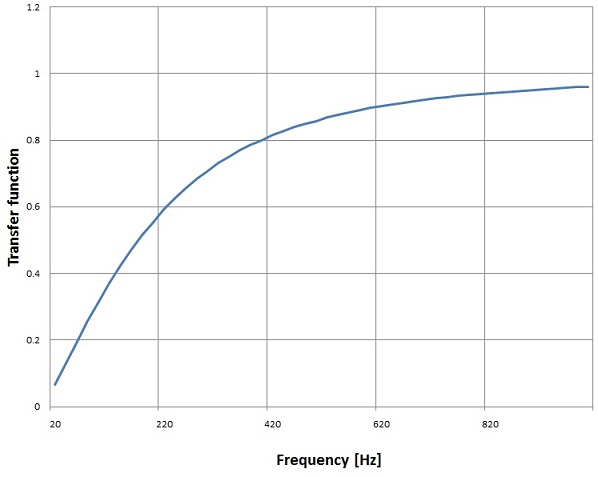
With a sampling frequency of 10 kHz and a cut off frequency of 300 Hz this filter creates this transfer function between 20 Hz and 1000 Hz:
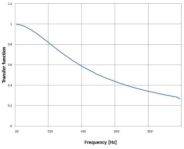
The transfer function of the real RC element in the frequency domain is:
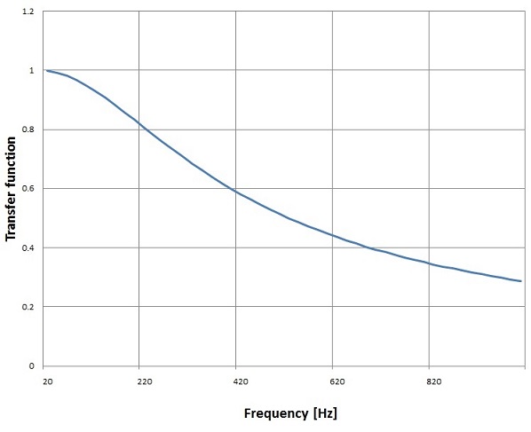
Almost no diffenence. That’s very close
High pass filter
The next step would be a high pass filter. In analogue technique that would look like:
Its transfer function:
Or in the Laplace domain:
The transformation into the z domain is similar to the above one.
Now digital filter parameters are:

If you compare these parameters with the parameters of the low pass filter, you might be astonished. There is no big difference. Only the enumerator is slightly different. Both values are additionally divided by T* and the sign of b1 is opposite to the sign of b0. That’s really no big difference. But the filter behaves completely different. It’s a high pass filter now and with a sampling frequency of 10 kHz and a cut off frequency of 300 Hz this filter creates this transfer function between 20 Hz and 1000 Hz:
The demo project consists of one main window. It processes a short sample signal (red curve) and displays the filtered signal (blue curve) the cut off frequency, sampling frequency and signal frequency can be set.
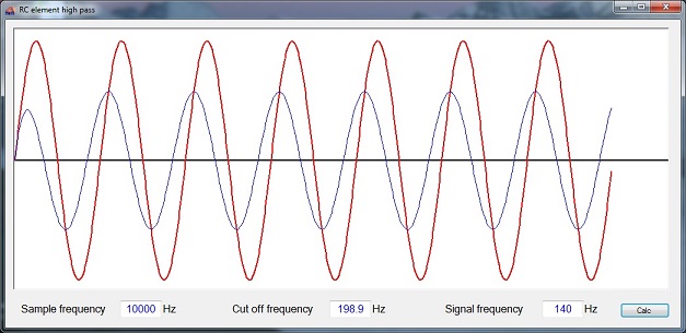
C# Demo Project RC element filter