

and in C# it looks like:
public void
CalcDFT(int N)
{
{
int k, n;
TKomplex w;
if (N > 0)
{
c[0].real = c[0].real / 2;
c[0].imag = c[0].imag / 2;
}TKomplex w;
if (N > 0)
{
for (k = 0; k < N; k++)
{
}{
c[k].real
= 0;
c[k].imag = 0;
for (n = 0; n < N; n++)
{
c[k].real = c[k].real / (double)(N) * 2.0;
c[k].imag = -c[k].imag / (double)(N) * 2.0;
}c[k].imag = 0;
for (n = 0; n < N; n++)
{
w.real = Math.Cos((double)(2.0 * Math.PI
* (double)(k * n)
/ (double)(N)));
w.imag = -Math.Sin((double)(2.0 * Math.PI * (double)(k * n) / (double)(N)));
c[k] = ksum(c[k], kprod(w, y[n]));
}w.imag = -Math.Sin((double)(2.0 * Math.PI * (double)(k * n) / (double)(N)));
c[k] = ksum(c[k], kprod(w, y[n]));
c[k].real = c[k].real / (double)(N) * 2.0;
c[k].imag = -c[k].imag / (double)(N) * 2.0;
c[0].real = c[0].real / 2;
c[0].imag = c[0].imag / 2;
 )
)The source of this standard implementation can be found in the Visual C# project DFT_std.
The functions ksum() and kprod() are simple functions for complex addition and multiplication
public TKomplex
ksum(TKomplex
a, TKomplex
b)
{
{
{
TKomplex res;
res.real = a.real + b.real;
res.imag = a.imag + b.imag;
return (res);
}res.real = a.real + b.real;
res.imag = a.imag + b.imag;
return (res);
{
TKomplex res;
res.real = a.real * b.real - a.imag * b.imag;
res.imag = a.real * b.imag + a.imag * b.real;
return (res);
}res.real = a.real * b.real - a.imag * b.imag;
res.imag = a.real * b.imag + a.imag * b.real;
return (res);
We build the look up table with:
for (k = 1; k < N; k++)
{
we[k].real
= Math.Cos((2.0
* Math.PI
* (double)(k) / (double)(N)));
we[k].imag
= -Math.Sin((2.0
* Math.PI
* (double)(k) / (double)(N)));
}
public void
CalcDFT() // Quick
and lean Fourier transformation
{
{
int k, n;
if (N > 0)
{
}if (N > 0)
{
for (k = 0; k < N; k++)
{
c[0].real = c[0].real / 2;
c[0].imag = c[0].imag / 2;
}{
c[k].real
= 0;
c[k].imag = 0;
for (n = 0; n < (N - 1); n++)
{
c[k].real = c[k].real / N * 2;
c[k].imag = -c[k].imag / N * 2;
}c[k].imag = 0;
for (n = 0; n < (N - 1); n++)
{
c[k]
= ksum(c[k], kprod(we[(k * n) % N], y[n]));
}c[k].real = c[k].real / N * 2;
c[k].imag = -c[k].imag / N * 2;
c[0].real = c[0].real / 2;
c[0].imag = c[0].imag / 2;
The code to this implementation is in DFT_lean.
We have a complex multiplication and a complex addition in our algorithm. So let’s have a look at them. First the multiplication we[x] * y[n]. That looks like
(we[x].re * y[n].re - we[x].im * y[n].im) + j(we[x].re * y[n].im + we[x].im * y[n].re)
y[n].im is always 0 and therefore the second and the third part are also 0 and our complex multiplication reduces to
(we[x].re * y[n].re) + j(we[x].im * y[n].re)
And that means
y[n].re * cosine(x) + j(y[n].re * sine(x))
That looks quite like ak and bk of the main clause. In the following addition we just have to sum the real parts and the imaginary parts. So there is no mixing of imaginary and real part in the complete calculation and finally we get the ak part in the real part of ck and the bk part in the imaginary part of ck and we can forget about all the complex stuff
With the limitation that the input sequence does not contain imaginary numbers we can implement the Fourier transformation without complex numbers:
public
void CalcDFT()
{
{
int
k, n;
if (N > 0)
{
}if (N > 0)
{
for
(k = 0; k < N; k++)
{
a[0] = a[0] / 2;
b[0] = b[0] / 2;
}{
a[k]
= 0;
b[k] = 0;
for (n = 0; n < (N - 1); n++)
{
a[k] = a[k] / N * 2;
b[k] = b[k] / N * 2;
}b[k] = 0;
for (n = 0; n < (N - 1); n++)
{
a[k]
=
a[k] + ((cosine[(k * n) % N] * y[n]));
b[k] = b[k] + ((sine[(k * n) % N] * y[n]));
}b[k] = b[k] + ((sine[(k * n) % N] * y[n]));
a[k] = a[k] / N * 2;
b[k] = b[k] / N * 2;
a[0] = a[0] / 2;
b[0] = b[0] / 2;
public
TFftAlgorithm(int
order)
{
{
int
k;
N = order;
y = new double[N + 1];
a = new double[N + 1];
b = new double[N + 1];
xw = new double[N + 1];
sine = new double[N + 1];
cosine = new double[N + 1];
cosine[0] = 1.0; // we don't have to calculate cos(0) = 1
sine[0] = 0; // and sin(0) = 0
for (k = 1; k < N; k++) // init vectors of unit circle
{
}N = order;
y = new double[N + 1];
a = new double[N + 1];
b = new double[N + 1];
xw = new double[N + 1];
sine = new double[N + 1];
cosine = new double[N + 1];
cosine[0] = 1.0; // we don't have to calculate cos(0) = 1
sine[0] = 0; // and sin(0) = 0
for (k = 1; k < N; k++) // init vectors of unit circle
{
cosine[k]
= Math.Cos((2.0
* Math.PI
* (double)(k) / (double)(N)));
sine[k] = Math.Sin((2.0 * Math.PI * (double)(k) / (double)(N)));
}sine[k] = Math.Sin((2.0 * Math.PI * (double)(k) / (double)(N)));
This implementation is in the project DFT_lean_quick.
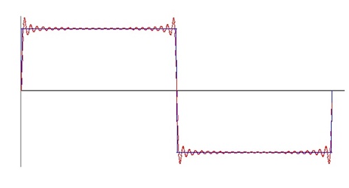
Whit the rectangle signal the result should look like this:
For the analytic Fourier transformation of the used sample signals see Fourier transformation
C# Demo Projects to Fourier transformation
Java Demo Project to Fourier transformation