

The first order Goertzel algorithm is a faster way to perform a Discrete Fourier Transformation. It’s disadvantage is a higher inaccuracy than the classical DFT algorithm has. That’s the price for the speed

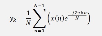
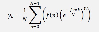
Based on the equation of the Fourier transformation
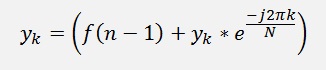
The first order Goertzel algorithm is built on the convolution of x[n] and an additional signal h[n] and ends, after a hell of a complicate explanation
, in the simple formula: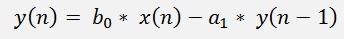
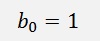
with:
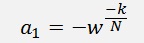
and
The implementation of this into a Fourier transformation I first time found in a very interesting book about Matlab. It basically looked like
a1 = -exp(1i*2*pi*k/N);
y = x(1);
for n = 2:N
y = x(n) - a1*y;
end
y = -a1*y;
O.k. we don’t analyse this syntax now
The signal path to this algorithm looks like :
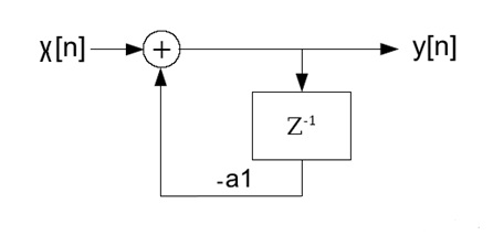
Principally that’s a system of first order containing a delayed feedback loop. The same algorithm in C looks like this
for
(k = 0; k < N; k++)
{
c[k].real
= y[0].real;
c[k].imag
= y[0].imag;
w.real
= -Math.Cos((double)(2.0
* Math.PI
* (double)(k)
/ (double)(N)));
w.imag
= Math.Sin((double)(2.0
* Math.PI
* (double)(k)
/ (double)(N)));
for
(n = 1; n <= N; n++)
c[k]
=
kdiff(y[n], kprod(c[k], w));
c[k] =
kprod(c[k], w);
c[k].real
= -c[k].real / (double)(N)
* 2.0;
c[k].imag
= -c[k].imag / (double)(N)
* 2.0;
}
With the complex operations
public
TKomplex
kdiff(TKomplex
a, TKomplex
b)
{
TKomplex
res;
res.real
= a.real - b.real;
res.imag
= a.imag - b.imag;
return
(res);
}
public
TKomplex
kprod(TKomplex
a, TKomplex
b)
{
TKomplex
res;
res.real
= a.real * b.real - a.imag * b.imag;
res.imag
= a.real * b.imag + a.imag * b.real;
return
(res);
}
Somehow I had the feeling that I have seen something like
already somewhere else… There is this thing about the polynomial
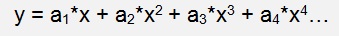
and its calculation like

If I implement this in a small loop, it almost looks like the formula above already. But a Fourier transformation does not look like this polynomial. The formula of the Fourier transformation is:
O.k.
But there is a way to bring this into a polynomial. The expression
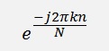
is a complex vector of the length 1 that spins around the unit circle. In the complex calculation we can say
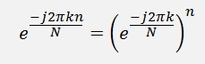
And the Fourier transformation can be written like
And that can be written as a polynomial
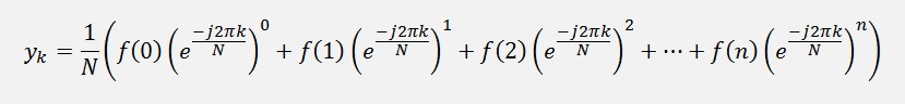
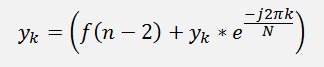
If I put this into a loop it starts like:
and goes on like
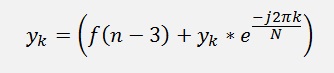
and
and
Till we are at f(0)
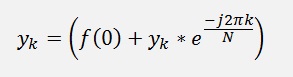
And theoretically
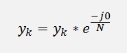
to finish this polynomial.
In the special case of the Fourier components this last term can be skipped as e0 = 1
Implemented in C this looks like
for
(k = 0; k < N; k++)
{
c[k].real
= y[N].real;
c[k].imag
= y[N].imag;
w.real
= Math.Cos((double)(2.0
* Math.PI
* (double)(k)
/ (double)(N)));
w.imag
=
-Math.Sin((double)(2.0
* Math.PI
* (double)(k)
/ (double)(N)));
for
(n = N - 1; n > 0; n--)
c[k]
=
ksum(y[n], kprod(c[k], w));
c[k].real
= c[k].real / (double)(N)
* 2.0;
c[k].imag
= -c[k].imag / (double)(N)
* 2.0;
}
That looks quite similar to the Goertzel algorithm already. But there are 3 points that differ:
1. w is of opposite sign
2. in the inner loop the indexing n starts at N-1 instead of 1. That means we work from the backside.
3. In the loop we have an addition instead of a subtraction.
Now the big question is: What does that mean? If I run into the other direction in my loop, that’s no difference for the addressing of the samples y[n]. They are still the same. But w is a complex vector. If we start at 0 whit n and increase it till N, w will spin counter clockwise. If we run into the other direction starting at N-1 and decreasing n till 1, w will spin clockwise. and that has some impact. Additionally we do not start at the same value of w. We start at
Instead of
This is basically the conjugate-complex value of w. Fortunately with this starting value w will spin clockwise automatically as it has a negative imaginary part
And finally: As we run into the other direction, the loop does not end at e0 and we cannot just skip the last term. With this modification the algorithm becomes like this
for
(k = 0; k < N; k++)
{
c[k].real
= y[0].real;
c[k].imag
= y[0].imag;
w.real
= Math.Cos((double)(2.0
* Math.PI
* (double)(k)
/ (double)(N)));
w.imag
= Math.Sin((double)(2.0
* Math.PI
* (double)(k)
/ (double)(N)));
for
(n = 1; n <= N; n++)
c[k]
=
ksum(y[n], kprod(c[k], w));
c[k] =
kprod(c[k], w);
c[k].real
= c[k].real / (double)(N)
* 2.0;
c[k].imag
= -c[k].imag / (double)(N)
* 2.0;
}
But still: The Goertzel algorithm does not work with the conjugate-complex of e-jx. It uses the negative value of it and subtracts this instead of adding it. Because of this finally the real part of the Fourier components becomes negative and has to be negated at the end of the loop. Now the algorithm looks like this:
for
(k = 0; k < N; k++)
{
c[k].real
= y[0].real;
c[k].imag
= y[0].imag;
w.real
=
-Math.Cos((double)(2.0
* Math.PI
* (double)(k)
/ (double)(N)));
w.imag
= Math.Sin((double)(2.0
* Math.PI
* (double)(k)
/ (double)(N)));
for
(n = 1; n <= N; n++)
c[k]
=
kdiff(y[n], kprod(c[k], w));
c[k] =
kprod(c[k], w);
c[k].real
= -c[k].real / (double)(N)
* 2.0;
c[k].imag
= -c[k].imag / (double)(N)
* 2.0;
}
And this is the Goertzel algorithm. Derived from a polynomial calculation with some small modifications we got the same algorithm
The main goal of the Goertzel algorithm is the calculation speed. It has to calculate much less sine and cosine values than the standard implementation of the DFT and therefore it works quite a bit faster. But in my article about the DFT I found a way to speed up the DFT algorithm even a bit more
And there is disadvantage: If we have a big amount of samples N will be big as well and due to that w will have a very small angle that has to be multiplied many, many times. A very small imaginary part has to be processed with a, compared to the imaginary part, big real part many times. That can cause a loss of accuracy of this calculation.
Run on a 32 bit system with less accuracy in the floating point numbers it even can become unstable and crash at a high amount of samples because the sine value of w will become 0.
For the analytic Fourier transformation of the used sample signals see Fourier transformation