

The Autoencoder is a usually not very deep neura netl (see Backpropagation for a detailed description) with a symmetric structure and reduced number of nodes in the middle. An important difference to a classic neural net is the fact, that, even though from the viewpoint of a neural net, there is the input layer on the left side (X) and the output layer on the right side (Y). The real output of the Autoencoder is the centre layer and the output layer of the neural net is set equal to the input layer for training.
The Autoencoder basically replicates the input data to the output output and yields the resulting data in the centre layer.
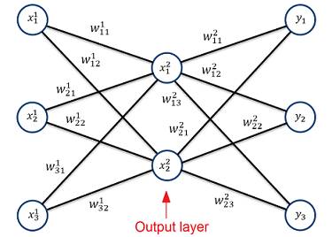
The simplest form of an Autoencoder with just 3 layers
That means for the training of an Autoencoder the target is to minimize the difference between the input values and the output values y1 ≌ x1, y2 ≌ x2…
If the training has successfully converged, the Autoencoder is capable to convert the input data into data of less features, represented in the middle layer, and rebuild the original data from this reduced data in the output layer. That means the data in the reduced centre layer still contains all the information (at least the most part of it) contained in the original data. That’s quite cool

In this form the Autoencoder does not use nonlinear activation functions like a Sigmoid function. It works absolutely linear.
And so on…
(note the indexing: x2 is not x to the power of 2. It’s just the index 2)
An important point is, the fact that the Autoencoder does not use any offsets as are used in most other neural nets.
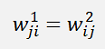
To perform a data reduction on a data set before it can be processed in a neural net, the autoencoder must be modified a bit. There must be some parameter sharing the way that the matrix W1 will be equal the transposed matrix W2 (see Matrix calculations for a detailed description)
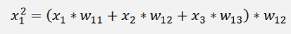
That means for the mathematical derivation the neural net with 3 layers should look like
Starting on the right side, the w-parameters on the left side must be mirrored from the right side in the way the matrix W1 will be the transposed matrix W2.
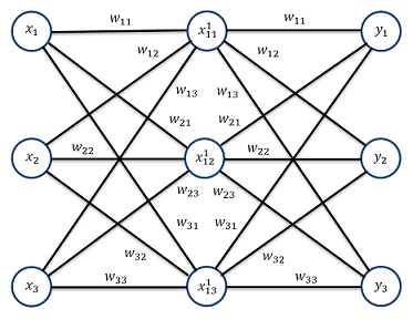
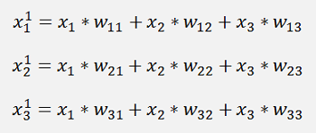
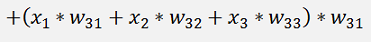
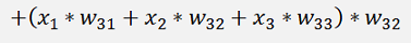
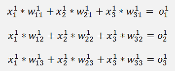
In this net we have
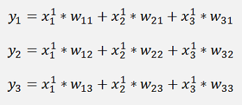
and
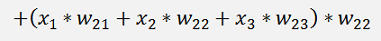
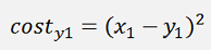
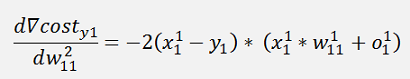
The complete equation for the output y1 becomes:

And with the cost function
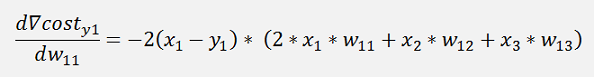
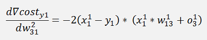
And the gradient of this with respect to w is:
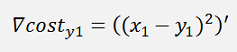
Where ∇cost is a vector with 3 rows here:
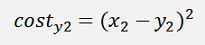
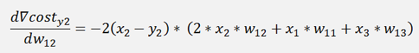
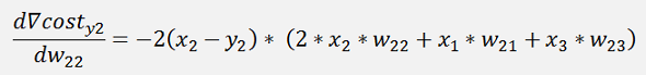
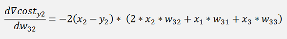
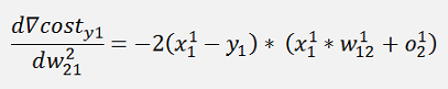
The same for y2:
And the cost:
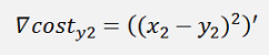
The gradients:
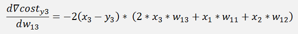
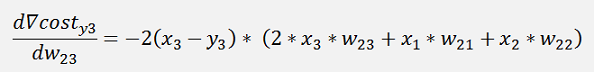
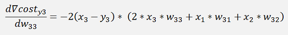
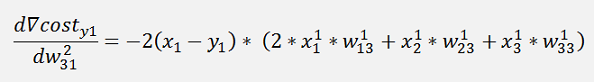
In the same manner we get for y3:
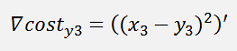
The gradients:
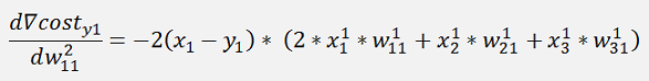
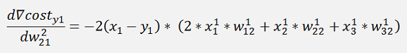
This is the pure mathematical formulation. In the implemented net there is one little difference: If we refer to the left side for the w parameters which is the input layer of the net. There the indexing is not like this. The parameter w12 is in reality w21 and w13 is w31 and so on. And that means the formulation for the implementation would be:
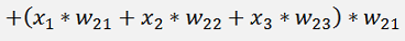
In these formulations there is the output of the middle layer. As
and we can rewrite
And so on… This is the formulation as it is usually mentioned in the literature if it comes to parameter sharing. They say: To train a neural net with parameter sharing is similar to train a net without parameter sharing. Just add the shared parameter to the derivation as many times it is shared. I think the situation is not really that simple

With this formulation we get the w-parameters of the output layer. These must be copied to the w-parameters of the input layer like
This is the way the Autoencoder must be trained.
In a c# the backward propagation procedure becomes:
private void BackwardProp(double[] x, double[] y)
{
int i, j, k;
TLayer rightLayer = net.ElementAt(layers - 1); // actual computed layer
TLayer leftLayer = net.ElementAt(0); // actual computed layer
double[] actX = new double[x.Length];
for (j = 0; j < rightLayer.featuresOut; j++)
{
costSum = costSum + ((y[j] - rightLayer.o[j]) * (y[j] - rightLayer.o[j]));
}
for (i = 0; i < rightLayer.featuresIn; i++)
{
for (k = 0; k < rightLayer.featuresOut; k++)
{
rightLayer.deltaW[i, k] += (rightLayer.w[i, k] * x[k] + leftLayer.o[i]) * (y[k] - rightLayer.o[k]);
}
}
}
(I used the Backpropagation algorithm and modified it)
And the UpdateValues function must be modified to copy the values of the right layer to the left layer:
private void UpdateValues()
{
int k, l;
TLayer rightLayer = net.ElementAt(layers - 1);
TLayer lefttLayer = net.ElementAt(0);
for (k = 0; k < rightLayer.featuresOut; k++)
{
for (l = 0; l < rightLayer.featuresIn; l++)
{
rightLayer.w[l, k] = rightLayer.w[l, k] + rightLayer.deltaW[l, k] / samples * learning_rate;
// copy the values of the right layer to the left layer
lefttLayer.w[k, l] = rightLayer.w[l, k];
}
}
}
The ForwardPropagation function can be left as it is.
Now there is one more point: The Autoencoder is relatively sensitive to data with big variation. Therefore it is wise to normalize the data before processing it in the Autoencoder and I did so in my demo project.
Now, to use this Autoencoder consider: There is a data set to train a neural net and there is a target data to be processed later on by this neural net. The procedure is to train the Autoencoder with the taining data set. When the Autoencoder has converged and the training is successfully finished, each sample of the training data set must be processed by the Autoencoder. The output values of the centre layer of this processing are the reduced data and must be stored in a new data set. This is the reduced training data set.
The reduced training data set is used to train the final neural net which is configured for the reduced data.
A target data sample must be normalized by the same parameters the training data set was normalized. Then the normalized data must be processed by the left part of the Autoencoder which is basically the multiplication of the data sample by the matrix W of the trained Autoencoder. That reduces the data sample to the size the final neural net is set up for. Like this it can be processed by the trained neural net in a forward propagation as it is usually done.
In my demo project I use the Iris data set as I already used it in most of all the other algorithms. The Iris data set is surely not the best choice to demonstrate an Autoencoeder. But it is a compact little data set. That makes it quite handy to use
This data set contains 150
samples of Iris flower data of 3 different flower types. Each sample
consists of 4 features. Of this data set I use a training data set of
135 samples. The last 5 samples of each flower I use as test data.
There are 3 C# projects. The Autoencoder reduces the 4 features to 2
features and saves this new data set in the file reduceddata.csv and
the values of the W matrix and normalisation parameters in the file
autoencoderdata.json in the program directory.The reduced data set is used to train the Backpropagation_Iris_reduced application. This is basically the same application as the Backpropagation application in the article Backpropagation. I just renamed it to avoid confusion.
In BackpropagationReducedTest I entered the W values of the trained neural net from the Backpropagation application and use the autoencoderdata.json for the data normalisation and reduction. In this application the test data is loaded, each sample is normalized and multiplied by the matrix W of the Autoencoder and finally processed by the neural net set up with the trained w values and offsets.
The Autoencoder I had to initialise a bit different from how I made it with the other neural nets. To get the Autoencoder to converge I could not initialise the w values with just a fixed value. I made it like:
for (j = 0; j < featuresOut; j++)
{
for (k = 0; k < featuresIn; k++)
{
w[k, j] = -0.4 + 0.4 * k;
}
}
{
for (k = 0; k < featuresIn; k++)
{
w[k, j] = -0.4 + 0.4 * k;
}
}
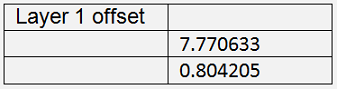
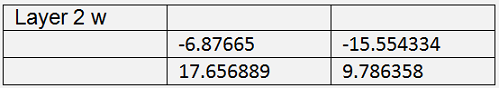
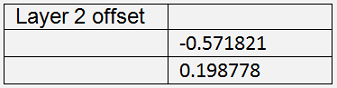
With this initialisation it gets the parameters
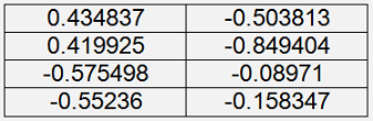
With the cost = 0.047
The training of the neural net in the Backpropagation_Iris_reduced application gets
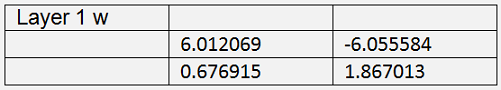
The cost = 0.047 is quite a bit higher than the one in Backpropagation with the full data set. That shows already that the data reduction has its disadvantages: There is some part of information that gets lost. That cannot be avoided. But with a bigger data set this loss will be smaller
With these parameters entered in the application BackpropagationReducedTest 14 of the 15 test samples are recognized correct. But the last sample is wrong.
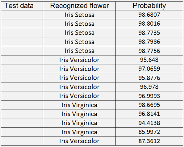
It says the last sample is a Iris Versicolor but in fact it is a Iris Virginica. The mean probability for the correct recognised flowers is not too high as well. That shows that obviously not all the information was transferred into the reduced data set. The Autoencoder does some kind of filtering. It reduces the variation in the data. The more the data is reduced the more variation is reduced. That’s a bit a disadvantage. But not all the information of a data set is needed all the time. Sometimes a little loss can be afforded in order to reduce the amount of data to compute.
The Autoencoder is a cool algorithm for such a data reduction. It is different from the Principal Component Analysis that rotates the coordinates system and offers the possibility to neglect data that does not carry much information. The Autoencoder takes all features and packs them into a smaller number of values. That’s another cool approach
There are 3 applications as demo projects. First the Autoencoder to reduce the data. Then the Backpropagation algorithm to train the neural net with the reduced data and finally the reduced data test that uses 15 samples to test. The Autoencoder produces the file autoencoderdata.json, The Backpropagation algorithm produces Layer0.json and Layer1.json. These 3 files must be copied into the execution directory of the test application to test.