

For classification tasks in backpropagation algorithms (Backpropagation for a detailed description) it is quite common to use the soft max function as activation function in the last layer of the neural net. Classification means assigning a vector of input features like [x1, x2, x3,…,xn] to a class1, class2,.., classm. Whereas each input vector can be assigned to only one class. In a neural net this is mapped by an output layer of m outputs that yields an output vector of m elements of which exactly one element is 1 and all the others are 0.
The Iris data set is a classic example for such a classification. It maps the measurement of the flowers of 150 plants their class. There are 3 classes in the data set: Iris-setosa, Iris-versicolor and Iris-virginica. I use this data set similar to how I used it in the other algorithms. I take the last 5 samples of each class as test samples and the remaining 135 samples for the training.
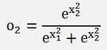
If the output is carried out as an array with 3 elements and we say
We get a classification task perfect for the soft max function.
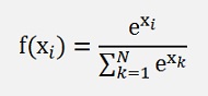
The soft max function is defined as
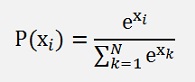
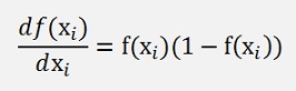
Similar to the sigmoid function the soft max function transforms the real value xi into a probability P(xi) with a value between 0 and 1. The big difference to the sigmoid function is that the soft max function takes all outputs into account in the denominator of the function.
If the soft max function is applied over all outputs, that yields a normalized vector and the sum of the results of all outputs is 1. That means the vector shows a distribution. With this distribution further processing like computing the cross entropy is possible. Which can be used as a cost function for training.
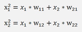
But first let’s have a deeper look on the soft max function. To see how to implement this soft max function into a backpropagation algorithm I start with a neural net with 1 basic layer and 2 input features similar to what I used in BackPropagation :
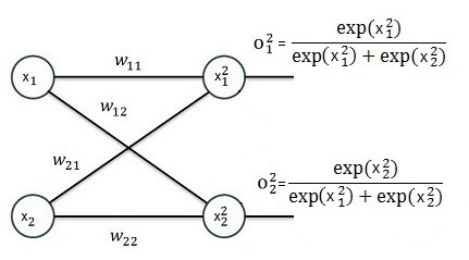
Whereas here x2 does not mean x to the power of 2. It’s just an indexing.
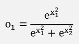
With
and
If we use the mean square deviation as Cost function, that’s still
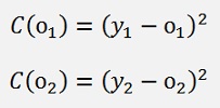
With xi as the input feature and yi the according element of the output class array of a sample.
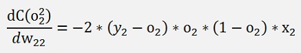
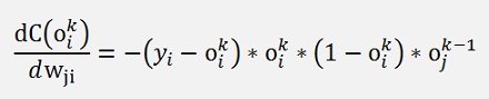
To compute the gradient of this cost function the derivation of C(oi) must be built with respect to wji.
With the quotient rule (see Differential calculus for a detailed description) we get for
the derivation
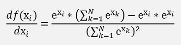
This can be expressed like
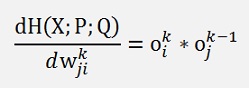
With this and applying the chain rule on the entire expression we get for the above net
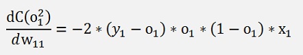
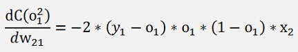
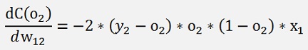
Or generally said
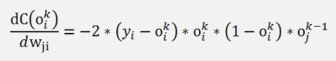
And the factor 2 can be neglected for convenience

So far the gradient in Backpropagation was a vector. Now, with soft max it becomes a matrix. That makes things slightly more complicate.
To be noted is that xj is the input of the above net. In a neural net whit more layers this is the output of the layer to the left. In my implementation that’s lastO.
For the gradient I defined an additional 2 dimensional matrix for the gradient in the Layer class
public double[,] gradientMatrix;
And implemented this formulation for the gradient in the backpropagation function like:
private void BackwardProp(double[] x, double[] y)
{
int i, j, k;
TLayer actLayer = layer.ElementAt(layers - 2); // actual computed layer
TLayer layerRight = layer.ElementAt(layers - 1); // next layer to the right of the actual one
double[] actX = new double[x.Length];
double[] lastO = new double[actLayer.o.Length];
for (j = 0; j < actLayer.o.Length; j++)
{
lastO[j] = actLayer.o[j];
}
actLayer = layer.ElementAt(layers - 1);
//last layer
for (j = 0; j < actLayer.featuresOut; j++)
{
costSum = costSum + ((y[j] - actLayer.o[j]) * (y[j] - actLayer.o[j]));
}
// compute the gradient for soft max
for (j = 0; j < actLayer.featuresIn; j++)
{
for (k = 0; k < actLayer.featuresOut; k++)
{
{
actLayer.gradientMatrix[j, k] = -lastO[j] * actLayer.o[k] * (1 - actLayer.o[k]) * (y[k] - actLayer.o[k]);
}
}
}
for (j = 0; j < actLayer.featuresIn; j++)
{
for (k = 0; k < actLayer.featuresOut; k++)
{
actLayer.deltaW[j, k] = actLayer.deltaW[j, k] + actLayer.gradientMatrix[j, k];
}
}
// all layers except the last one
if (layers > 1)
{
for (i = layers - 2; i >= 0; i--)
{
actLayer = layer.ElementAt(i);
layerRight = layer.ElementAt(i + 1);
if (i > 0)
{
TLayer layerLeft = layer.ElementAt(i - 1);
for (j = 0; j < layerLeft.o.Length; j++)
actX[j] = layerLeft.o[j]; }
else
{
for (j = 0; j < x.Length; j++)
{
actX[j] = x[j];
}
}
for (j = 0; j < actLayer.featuresOut; j++)
{
// compute the gradient for the other layers
actLayer.gradient[j] = 0;
if (!layerRight.isMatrixGradient)
{
for (k = 0; k < layerRight.featuresOut; k++)
{
actLayer.gradient[j] = actLayer.gradient[j] + (layerRight.gradient[k] * actLayer.dAct(actLayer.o[j]) * layerRight.w[j, k]);
}
}
else
{
for (k = 0; k < layerRight.featuresOut; k++)
{
actLayer.gradient[j] = actLayer.gradient[j] + (layerRight.gradientMatrix[k, j] * actLayer.dAct(actLayer.o[j]) * layerRight.w[j, k]);
}
}
// the delta for the learning
actLayer.deltaOffs[j] = actLayer.deltaOffs[j] + actLayer.gradient[j];
for (k = 0; k < actLayer.featuresIn; k++)
{
actLayer.deltaW[k, j] = actLayer.deltaW[k, j] + actLayer.gradient[j] * actX[k];
}
}
}
}
}
In the forward propagation I had to add the enumerator for the soft max function. That makes it a bit more complicate as well:
private double[] ForwardProp(double[] x)
{
int i, j, k;
TLayer actLayer = layer.ElementAt(0);
double[] actX = new double[x.Length];
for (i = 0; i < x.Length; i++)
{
actX[i] = x[i];
}
actLayer.calcSum = true;
for (i = 0; i < layers - 1; i++)
{
for (j = 0; j < actLayer.featuresOut; j++)
{
actLayer.x[j] = actLayer.offs[j];
for (k = 0; k < actLayer.featuresIn; k++)
{
actLayer.x[j] = actLayer.x[j] + actX[k] * actLayer.w[k, j];
}
actLayer.o[j] = actLayer.Act(actLayer.x[j]);
}
for (j = 0; j < actLayer.x.Length; j++)
{
actX[j] = actLayer.o[j];
}
actLayer = layer.ElementAt(i + 1);
}
// last layer
for (j = 0; j < actLayer.featuresOut; j++)
{
actLayer.x[j] = 0;
for (k = 0; k < actLayer.featuresIn; k++)
{
actLayer.x[j] = actLayer.x[j] + actLayer.w[k, j] * actX[k];
}
}
double enumerator = 0;
for (j = 0; j < actLayer.featuresOut; j++)
{
enumerator = enumerator + Math.Exp(actLayer.x[j]);
}
for (j = 0; j < actLayer.featuresOut; j++)
{
actLayer.o[j] = Math.Exp(actLayer.x[j]) / enumerator;
}
return actLayer.o;
}
I used the project I implemented for my Backpropagation and just modified the respective lines, set up the neural net with 3 layers like
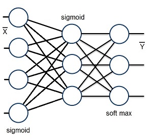
This is done in
tempRow = new TLayer(4, 3);
tempRow.InitSigmoid();
layer.Add(tempRow);
tempRow = new TLayer(3, 3);
tempRow.InitSigmoid();
layer.Add(tempRow);
tempRow = new TLayer(3, 3);
tempRow.InitSoftMax();
layer.Add(tempRow);
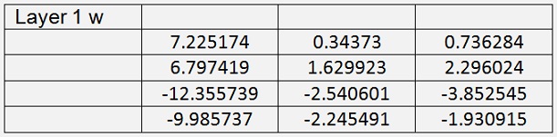
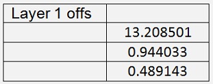
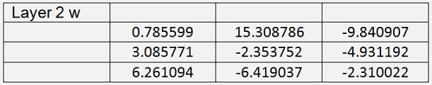
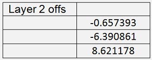
It would basically be possible to use just 2 layers. But the result with 3 layers is better. With this set up I got with 400000 iterations and a learning rate of 0.6
With a mean cost of 0.02
The test application with 15 test samples recognizes all samples correct with a mean possibility of 98.9 %
Using cross entropy as cost function
As the soft max function yields a distribution on the output of the neural net, the cross entropy (see https://en.wikipedia.org/wiki/Cross_entropy) as cost function. That looks quite complicate on the first glimpse, but in fact it isn’t
The cross entropy gives a measure how well a real distribution and its model fit together. Its basic formulation for a discrete case (what we actually have here) is:
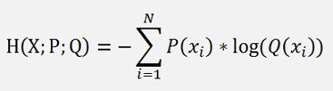
Whereas P(xi) is the real distribution and Q(xi) is the model that we are looking for and this model is the soft max probability:
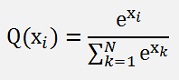
And xi is one element of the output feature vector of one data sample.
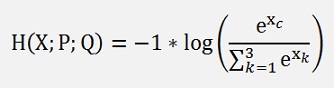
In a classification problem we have exactly one element in P(X) that is not 0. It’s the element of the index of the particular class and therefore the cross entropy becomes
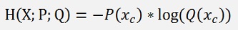
With c as the index of the class (that means if y2 = 1 then c = 2).
That means in the Iris data set the first sample is an Iris-setosa, its output feature vector Y = [1, 0, 0] and therefore the formula for its cross entropy becomes
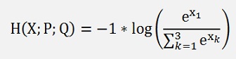
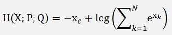
Or generally said
With c as the index of the output which is 1 and X the input of the soft max layer.
And this cross entropy for the output index c where the class label is 1 is the cost function that is used for training.
An important detail is that so far in backpropagation algorithms the cost function was defined one per output. But now as every output is linked to every other output in the enumerator of the soft max function, there is one cost function valid for all outputs. So for the gradient we have to differentiate this one cost function with respect to all indexes of wji.
For this differentiation the cross entropy formulation is reformed like:
And remember:
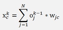
And if we want the differentiate the cost function with respect to a wji with I <> c, the differentiation of xc becomes 0.
So there are 2 cases for the index in wji:
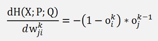
If i = c:
If I ≠ c:
This can be simplified a bit if we consider yc = 1 and all other yi = 0:
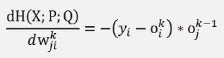
If you compare this with the gradient for the mean square deviation cost function from above:
Only the part
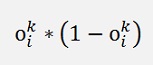
has vanished. All the rest is the same
So there is just a very small modification needed to convert the mean square deviation as cost function to a cross entropy. Just delete these two expressions and in the backpropagation routine the line for the gradient becomes
actLayer.gradientMatrix[k, j] =-lastO[k] *
(y[j] -
actLayer.o[j]);
Instead of
actLayer.gradientMatrix[j, k] = -lastO[j] *
actLayer.o[k] * (1 - actLayer.o[k]) * (y[k] - actLayer.o[k]);
With the cross entropy as cost function the algorithm behaves quite different from the above one. That’s why I introduced different learning rates for the different layers. I use 0.6 for the first 2 layers and 0.01 for the soft max layer. That works slightly better than using the same for all layers.
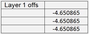
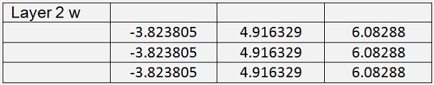
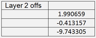
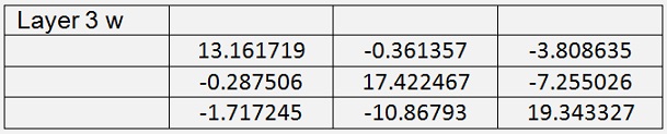
With this and with 200000 iterations I got
With a mean cost of 0.015
For comparison this cost is computed by mean square deviation.
The test application recognizes all 15 test samples correct with the mean possibility of 99.44 %. Compared to the 98.9 % with mean square deviation that’s quite a bit closer to 100 % even though the cost of the training was a bit higher
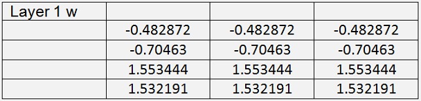
The demo project consists of one main window.
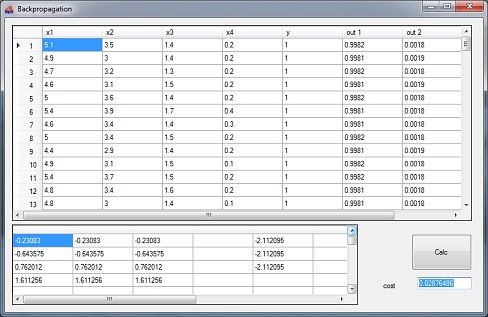
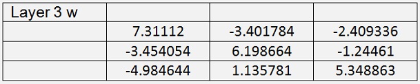
In the upper string grid there is the input data and the computed outputs and in the lower string grid there are the trained parameters for w on the left and the offsets on the right side. Pressing "calc" starts the training. That takes something around 2 minutes on my computer.
It creates 3 json file containing the trained values of the net. They are stored in the application directory with the file names Layer0.json … Layer3.json. Theses 3 json files must be copied into the application directory of the test application for testing.