

Solving an optimisation problem is often a question of finding a minimum or maximum of a function with more than one input variable. The minimum or maximum of a function is there where it’s first differentiation is 0. One way to solve this problem is to use the Gradient descend method.
Another interesting approach is Isaac Newton’s method. Newton developed a method to find the real roots of a polynomial (see Newton Maehly). The idea for his optimisation method with more than one input variable is based on this algorithm.
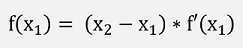
In the Newton Maehly algorithm the basic idea is to introduce a linearization of the polynomial function by the use of the differentiation of it.

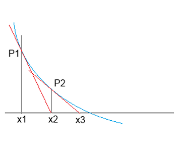
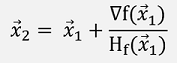
With this linearization he can approximate:
Or to move into the direction of the nearest root:
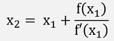
That will most probably not meet the nearest root, but x2 will already be closer to it and from there in the same manner to x3 brings us another step closer.
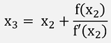
This sequence is repeated until f(xn) is close enough to 0.
In an optimisation problem we don’t want to find the roots of the function itself, but of its differentiation and for this the formulation becomes:
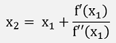
We have to use the first and the second differentiation of the function (in case it can be differentiated twice). That would be the approach if there would be just one input variable. If we have more than one input variables, things become a little more complicate
If there are more than one input variables, these input variables are represented by a vector:
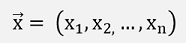
Now the differentiation of this vector is another vector where one element is the differentiation of the above function with respect to one variable:
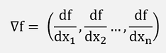
This is the so called Gradient of the function f(x1, x2, …, xn) and usually the Nabla operator ∇ is the sign for this Gradient.
The second differentiation of the function f(x1, x2, …, xn) becomes a matrix in the form
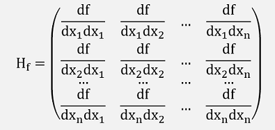
This matrix is the Hessian matrix.
With these we could say
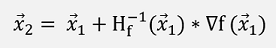
But as there is no division defined for a matrix, that does not work. We have to build the inverse of the matrix H and use:
This formulation is quite often related to the Tailor approximation. But I would say it has not too much to do with that
In a small sample project, I implemented the search for the saddle point of the function
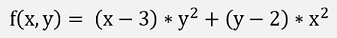
It has a saddle point at x = 1.832 and y = 1.4367, where f’(x,y) = 0
The graph of the function looks like this:
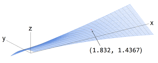
It bends in all directions and the saddle point is the little red dot. It does not look too interesting. But o.k., it’s just a sample
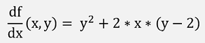
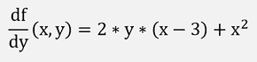
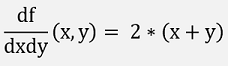
The first differentiations are:
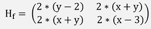
The second differentiations are:
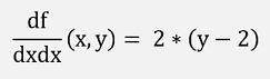
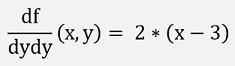
And with this the Hessian Matrix:
This implemented in two small C# functions:
void fillGradient(double x, double y)
{
gradient[0] = y * y + 2 * x * (y - 2);
gradient[1] = 2 * y * (x - 3) + x * x;
}
void fillHessian(double x, double y)
{
hessian[0, 0] = 2 * (y - 2);
hessian[0, 1] = 2 * (x + y);
hessian[1, 0] = 2 * (x + y);
hessian[1, 1] = 2 * (x - 3);
}
And for the update to the next point:
void update_rise()
{
fillGradient(x, y);
fillHessian(x, y);
// p(x,y) = p(x,y) - hessian^-1 * gradient
m.InitMatrix(hessian);
m.Invert();
delta = m.Mult(m.inv, gradient);
x = x - delta[0];
y = y - delta[1];
}
With
Matrix m = new
Matrix(features);
The class Matrix is a small implementation of the Matrix inversion by Cramer (see Inverse Matrix) and Matrix multiplication.
With this and the declarations
double[] gradient = new double[features];
double[,] hessian = new double[features, features];
double[] delta = { 10, 10 };
double x = 4;
double y = 4;
A little loop can be implemented like:
while ((Math.Abs(delta[0]) > 1E-5) && (Math.Abs(delta[1]) > 1E-5))
{
update_rise();
}
This loop finds the saddle point within 6 iterations.
The sample project consits of one main window:
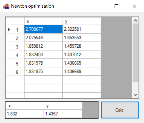
Pressing the button <Calc> runs the algorithm. In the upper Grid the computed values for x and y are printed for each iteration. At the end of the loop the result for x and y is displayed in the lower grid.