Natural splines

Interpolation by Natural splines

For the spline interpolation one interpolation function is calculated for each interval between two supporting points.

If we have for instance a set of 6 supporting points, the interpolation would look like this:

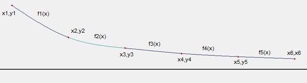
To this 6 supporting points we get 5 different functions f₁(x), f₂(x)..f₅(x). For x₁ =< x < x₂ y = f₁(x), for x₂ =< x < x₃ y = f₂(x) and so on.

For each of these intervals one cubic polynomial function is calculated like:

for the interval starting at xi and ending at xi+1 and x as the interpolation variable. That means in opposite to the other interpolation algorithms we do not get just one interpolation function but N-1 for N supporting points. And we finally have to switch these functions when we build the interpolation graph.

To make sure that the wave shapes of all this intervals fit together and build a smooth wave shape, there are some conditions to be fulfilled:

a) The graph of the functions shall meet all the supporting points

p_i(x_i ) = y_i for i = 1 to N

b) The graph shall not have a jump discontinuity at the supporting points

p_i (x_i ) = p_i-1(x_i ) for i = 2 to N-1

c) There shouldn’t be any break-points at the supporting points

p'_i (x_i ) = p'_i-1 (x_i ) for i = 2 to N-1

d) The bending of the graph shall be the same on both sides of the supporting points

p''_i (x_i ) = p''_i-1 (x_i ) for i = 2 to N-1

With N as the number of supporting points.

From these conditions and the substitution h_i = x_i+1 - x_i the parameters a, b, c and d can be derived:

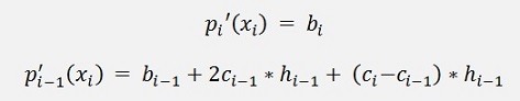
From condition a we get a_i = y_i. If x = x_i, then x – x_i = 0 and p_i(x) = a_i = y_i

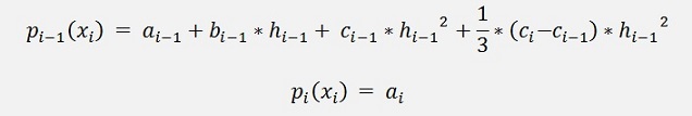
With the second deductions

and the substitution

inserted in the formulation of b

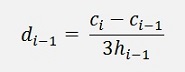
This resolved for d_i-1

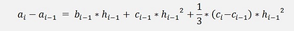
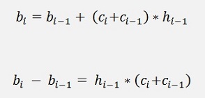
And with this we get from b

And both put together

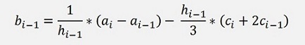
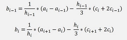
Resolved for b_i-1:

Or b_i:

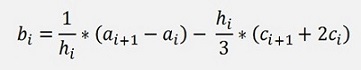
This will be the equation to compute b_i

And we’ll use further down

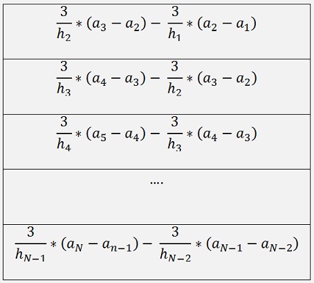
From c we get

(with the same substitution for di-1 as above)

Now we remember the 2 equations from above

And use them

Here we bring all the c terms on one side

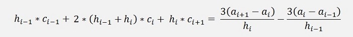
Now, there is a boundary condition for natural spines: The interpolated graph shall continue in a straight line on both ends. That means

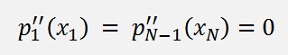
and

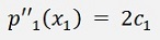
That means c₁ = 0 for natural splines.

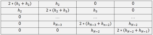
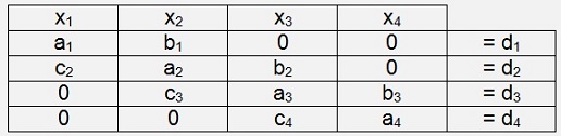
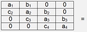
With this the equation leads to a matrix equation of the order N-2 for c_i with i = 2 ..n-1 and the matrix.

and the solution vector

This matrix equation solved yields c₂ to c_N-1. The first and the last c both are set as 0.

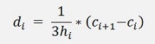
Now there is only d_i left and this we get from condition d

With these parameters each of the intervals between the supporting points can be interpolated now and at the end the pieces have to be put together to one graph.

The algorithm to calculate the parameters looks like:

public bool CalcParameters()
{
     int i, k;
     for (i = 0; i < order; i++) // calculate a parameters
     {
         a[i] = y_k[i];
     }
     for (i = 0; i < order - 1; i++)
     {
         h[i] = x_k[i + 1] - x_k[i];
     }

     // empty matrix for c parameters
     for (i = 0; i < order - 2; i++)
     {
         for (k = 0; k < order - 2; k++)
         {
              m[i, k] = 0.0;
              y[i] = 0.0;
              x[i] = 0.0;
         }
     }

     // fill matrix for c parameters
     for (i = 0; i < order - 2; i++)
     {
         if (i == 0)
         {
              m[i, 0] = 2.0 * (h[0] + h[1]);
              m[i, 1] = h[1];
         }
         else
         {
              m[i, i - 1] = h[i];
              m[i, i] = 2.0 * (h[i] + h[i + 1]);
              if (i < order - 3)
                   m[i, i + 1] = h[i + 1];
         }
         if ((h[i] != 0.0) && (h[i + 1] != 0.0))

y[i] = ((a[i + 2] - a[i + 1]) / h[i + 1] - (a[i + 1] - a[i]) / h[i]) * 3.0;

         else
              y[i] = 0.0;
     }
     if (gauss.Eliminate())
     {
         gauss.Solve();
         c[0] = 0.0; // boundry condition for natural splines
         for (i = 1; i < order - 1; i++)
              c[i] = x[i - 1];
         for (i = 0; i < order - 1; i++) // calculate b and d parameters
         {
              if (h[i] != 0.0)
              {

d[i] = 1.0 / 3.0 / h[i] * (c[i + 1] - c[i]);
b[i] = 1.0 / h[i] * (a[i + 1] - a[i]) - h[i] / 3.0 * (c[i + 1] + 2 * c[i]);

              }
         }
         return true;
     }
     else
         return false;
}

The part for the interpolation is

public void Interpolate(int order, int resolution)
{
     int i, k;
     double timestamp;
     for (i = 0; i < order - 1; i++)
     {
         for (k = 0; k < resolution; k++)
         {

timestamp = (double)(k) / (double)(resolution) * h[i];

yp[i * resolution + k] = a[i] + b[i] * (timestamp) + c[i] * Math.Pow(timestamp, 2) + d[i] * Math.Pow(timestamp, 3);
xp[i * resolution + k] = timestamp + x_k[i];

}
}
}

This is the basic algorithm for Natural Splines.

But, that’s not all. The Matrix equation to calculate the h parameters contains many elements that are 0 and due to this fact there can by an improvement to solve this equation :-)

Improvement of calculation speed by LU decomposition

To calculate the h parameters we have to solve a matrix equation of following structure:

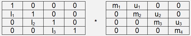
This is a tridiagonal matrix (at least as long as we don’t want to interpolate a periodic function). This special case of a matrix equation can be solved much quicker than by using the Gaussian elimination algorithm by using the LU decomposition of Durant Crout transforming the A matrix of the equation Ax = D into a lower triangular matrix and a upper triangular matrix as A = LU like.

Comparison of the parameters gives:

c₂ = l₁ * m₁
c₃ = l₂ * m₂
c₄ = l₃ * m₃

a₁ = m₁
a₂ = l₁ * u₁ + m₁
a₃ = l₂ * u₂ + m₂
a₄ = l₃ * u₃ + m₃

b₁ = u₁
b₂ = u₂
b₃ = u₃
b₄ = u₄

And from this for the elements:

l_i = c_i+1 / m_i
m_i+1 = a_i+1 – l_i * b_i
for i = 1 to N-1

To solve this equation we first extend the equation LUx = D by y and say LUxy = Dy (y is not the solution vector of the very top equation). This can be separated to Ly = D and Ux = y.

Ly = D looks like

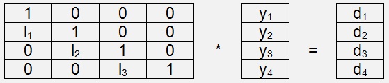
And resolving Ly = D gives

y₁ = d₁
y₁ * l₁ + y₂ = d₂
y₂ * l₂ + y₃ = d₃
y₃ * l₃ + y₄ = d₄

=> y₁ = d₁
=> y₂ = d₂ - y₁ * l₁
=> y₃ = d₃ – y₂ * l₂
=> y₄ = d₄ – y₃ * l₃

With this we basically have to implement 3 loops to solve the tridiagonal Matrix equation:

First loop:

m₁ = a₁
For i = 1 to n-1

l_i = c_i+1 / m_i

m_i+1 = a_i+1 – l_i * b_i

put into c code:

Second loop:

y₁ = d₁
for i = 2 to n

y_i = d_i – l_i-1 * y_i-1

In c code:

y_lu[0] = m.y[0];
for (i = 1; i < order; i++)
{
y_lu[i] = y[i] - l_lu[i - 1] * y_lu[i - 1];
}

Third loop:

x_n = y_n / m_n
For I = n-1 to 1
x_i = (y_i - b_i * x_i+1)/m_i
In c code:

if (Math.Abs(m_lr[order - 1]) > 1E-10)
     x[order - 1] = y_lu[order - 1] / m_lr[order - 1];
else
     calcError = true;
if (!calcError)
{
     for (i = order - 2; i >= 0; i--)
     {
         x[i] = (y_lu[i] - a[i, i + 1] * x[i + 1]) / m_lu[i];
     }
}

Now the first and second loop can be implemented in one if we separate the first term of the first loop and the last term of the second loop

m₁ = a₁
l₁ = c₂ / m₁
m₂ = a₂ – l₁ * b₁
For i = 2 to n-1
l_i = c_i+1 / m_i
m_i+1 = a_i+1 – l_i * b_i
y_i = d_i – l_i-1 * y_i-1
y_N = d_N – l_N-1 * y_N-1

So there remain 2 loops to solve the entire matrix equation and that takes a bit more than half as much calculation time as a Gaussian algorithm :-)

The final c code :

m_lu[0] = m.a[0, 0];
for (i = 0; i < order - 1; i++)
{
     if (Math.Abs(m_lu[i]) > 1E-10)
         l_lu[i] = m[i + 1, i] / m_lu[i];
     else
     calcError = true;
     m_lu[i + 1] = m[i + 1, i + 1] - l_lu[i] * m[i, i + 1];
}
y_lu[0] = m.y[0];
for (i = 1; i < order; i++)
{
     y_lu[i] = y[i] - l_lu[i - 1] * y_lu[i - 1];
}
if (Math.Abs(m_lr[order - 1]) > 1E-10)
     x[order - 1] = y_lu[order - 1] / m_lu[order - 1];
else
     calcError = true;
if (!calcError)
{
     for (i = order - 2; i >= 0; i--)
     {
         x[i] = (y_lu[i] - m[i, i + 1] * x[i + 1]) / m_lu[i];
     }
}

That's it

For Periodic splines see periodic splines

For End slope splines see end slope splines

C# Demo Projects to natural splines

Spline.zip

Spline_LU.zip

Java Demo Projects to natural splines

Splines.zip

Spline_LU.zip