

Gradient descent is an algorithm that is used for optimisation in the field of machine learning. It’s basic function is to search for the best approximation of a function with more than one independent input variables. These variables occur in linear form. So the function is multidimensional.
To find this best approximation the algorithm runs along the gradient descend of the function in the same way the Linear regression iterative. Only it does this for all dimensions at once.
I implemented an algorithm to approximate a multidimensional function with only linear input variables as a multi variable linear regression and another algorithm to search the minimum of a 2 dimensional function with 2 polynomials of second order as input. Therefore I generated some test data that build the square function of the surface of the lower part of a sphere and search the minimum of this sphere surface. That will be a bit further down. First there is the multi variable linear regression.
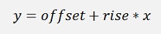
The linear regression for one single input variable x approximates a random number of supporting points (x,y) to a straight line with the formulation
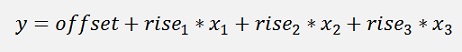
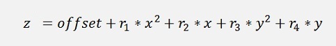
A multi variable linear regression does the same for more than one x and it approximates a plane. For a 3 dimensional input that would be:
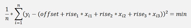
Here the values offset, r1, r2 and r3 shall be determined the way that the mean value of the deviations of the approximation at all supporting points (which are vectors now) in square becomes the smallest.
That means
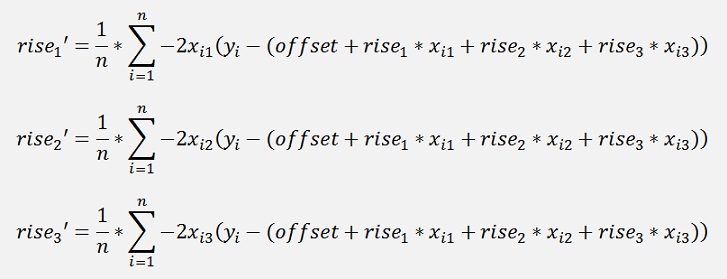
The offset must be processed separately (see Linear regression iterative). So there remain 3 unknown parameters r1, r2 and r3. For these the derivation must be built now:
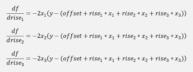
With this derivation a mean rise for each dimension is computed by the use of all supporting points like
And with this rise’ and the so called learning rate, the actual rise is adjusted:
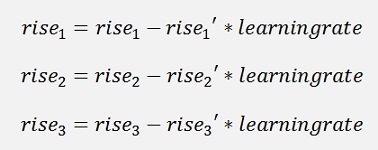
And as we have the factor 2 in all equations, this factor can as well be left away. That saves 3 multiplications each loop. The learning rate is usually something around 0.01. Its value depends on the number of samples.
In a C# function that’s:
{
int i, j;
double[] predictions = update_values(x, rise);
double[] d_rise = new double[features];
for (i = 0; i < features; i++)
{
d_rise[i] = 0;
for (j = 0; j < samples; j++)
{
d_rise[i] = d_rise[i] + x[j, i] * (y[j] - predictions[j]);
}
d_rise[i] = -d_rise[i] / samples;
}
for (i = 0; i < features; i++)
{
rise[i] = rise[i] - learning_rate * d_rise[i];
}
return rise;
}
with
double[] update_values(Collection<double[]> values, double[] rise)
{
double[] predictions = new double[samples];
double[] x;
for (int i = 0; i < samples; i++)
{
predictions[i] = 0;
x = values[i];
for (int j = 0; j < features; j++)
{
predictions[i] = predictions[i] + x[j] * rise[j];
}
predictions[i] = predictions[i] + offset;
}
return predictions;
}
The adjusting value is subtracted from the actual rise value because we are searching for the minimum and want to move downward the slope.
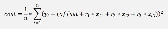
With this new rise the mean deviation square is computed. This deviation is often called cost and the function that computes it is the cost function
Or in a c# function:
double cost_function(Collection<double[]> values, double[] rise)
{
int i, j;
double cost = 0;
double[] predictions = update_values(values, rise);
double[] x;
double y;
cost = 0;
for (j = 0; j < samples; j++)
{
x = values[j];
y = x[features];
cost += (y - predictions[j]) * (y - predictions[j]);
}
cost = cost / samples / 2.0;
return cost;
}
I keep the data in a collection of arrays
Collection<double[]>
values = new Collection<double[]>();
And the last element in one array is the y value of one data point. The other values in the array are the input variables x1…xn.
If this 2 operations are done iteratively, the deviation, or cost, will decrease slowly till it gets to a minimum for the rise values.
double[] find_min(Collection<double[]> values, double[] rise, double learning_rate, int maxIers)
{
int count = 0;
double oldCost = -1;
double divCost = oldCost - cost;
double[] ret = new double[2];
while (Math.Abs(divCost) > 1e-5 && count < maxIers)
{
rise = update_rise(values, rise, learning_rate);
cost = cost_function(values, rise);
divCost = oldCost - cost;
oldCost = cost;
count++;
if (divCost < -0.001)
{
learning_rate = -learning_rate / 2;
}
}
return rise;
}
Now, similar to how I implemented it in Linear regression iterative the offset must be threatened separately.
I do the above minimum search for a starting offset of 0, correct it by the mean deviation (not the square of it) and check whether the next cost is small enough that we can say we found the real minimum cost.
offset = 0;
while ((Math.Abs(divCost) > 0.000001) && (count < 1000))
{
rise = find_min(data.values, rise, learning_rate, iterations);
divCost = oldCost - cost;
if (divCost < -0.001)
{
step = -step / 2.0;
}
lastCost = oldCost;
oldCost = cost;
cost_history[count] = cost;
offset = offset + mean_function(data.values, rise);
count++;
}
with
double mean_function(Collection<double[]> values, double[] rise)
{
int i, j;
double mean = 0;
double[] predictions = update_values(values, rise);
double y;
for (j = 0; j < samples; j++)
{
y = values.ElementAt(j)[features];
mean += (y - predictions[j]);
}
mean = mean / samples / 2;
return mean;
}
Now there is only one little problem: In the function update_rise there is a sum computed that can become quite big if the number of input data samples is big. This sum can produce an overflow. In some articles I saw ideas to normalize all the input data. But I personally do not like that too much I use another solution. Just summarize into a temporary variable and if this becomes big, divide it by the number of samples, add it to the final sum and set it back to 0. Then go on summarizing.
That looks like:
double[] update_rise(Collection<double[]> values, double[] rise, double learning_rate)
{
int i, j;
double[] predictions = update_values(values, rise);
double[] d_rise = new double[features];
double[] x;
double y;
double tempSum = 0;
for (i = 0; i < features; i++)
{
d_rise[i] = 0;
tempSum = 0;
for (j = 0; j < samples; j++)
{
x = values.ElementAt(j);
y = x[features];
tempSum = tempSum + x[i] * (y - predictions[j]);
if(Math.Abs(tempSum) > 1e6)
{
d_rise[i] = d_rise[i] - tempSum / samples;
tempSum = 0;
}
}
d_rise[i] = d_rise[i] - tempSum / samples;
}
for (i = 0; i < features; i++)
{
rise[i] = rise[i] - learning_rate * d_rise[i];
}
return rise;
}
Like that no overflow can happen and no complicate normalisation is required

In my sample project I use input data that was built by the function
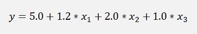
I set up 100 data samples and with this I got the approximation

That might look a bit strange on the first glimpse. But keep in mind this formulation is valid only for the 100 data samples. For these 100 samples the mean deviation is 6.24E-06. That’s quite close and the more data samples are used the closer the result gets to the origin function
The deviation distribution over all data samples looks like:
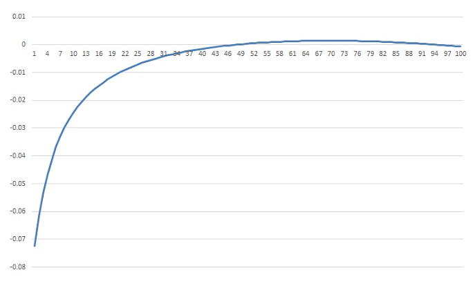
With the smaller values the deviation is a bit bigger and more or less in the middle (regarding the value of y) the deviation is the smallest.
In the sample application there is a data grid showing the input data x1..x3, y, f(x) which is the approximated y and the deviation between y and f(x) is displayed.
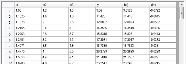
The input data is held in the data file data.csv. It’s a comma separated file containing only the data, no headers. The first 3 columns contain x1..x3 and the last column contains y. There is an excel sheet in the project folder that contains the same data. I used this to generate the data and to compare the result with this data.
If it comes to testing of an algorithm it’s often a question of useful test data. So the idea came to me to set up supporting points forming the lower part of a sphere and to find the lowest point of this sphere. The sphere has a radius of 4 and the centre point is at x = 3 and y=2 and the complete sphere gets an offset of 5 in z direction.
And as I use only the lower part of the sphere the formulation is
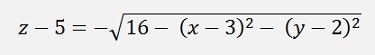
As the minimum will be the same for z and z2 and the root function is quite calculation intensive, I approximate z2
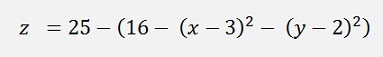
This is the formulation to compute the test data and its minimum will be 9 with x = 3 and y = 2.
Additionally I add a random value between -0-05 and +0.05 to get a small variation into the data.
To find the minimum of this function we first have to find the approximating function and with this we can search for the minimum.
The estimated function to approximate is:
And therefore the derivatives for the deviations are:
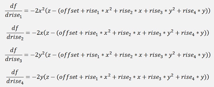
This and the function itself are the only difference to the algorithm from above. The factor 2 can be left away here again and that makes the following C# functions for the function values z2:
double[] update_values(Collection<double[]> values, double[] rise)
{
double[] predictions = new double[samples];
double[] x;
for (int i = 0; i < samples; i++)
{
x = values[i];
predictions[i] = offset + x[0] * x[0] * rise[0] + x[0] * rise[1] + x[1] * x[1] * rise[2] + x[1] * rise[3];
}
return predictions;
}
and
double[] update_rise(Collection<double[]> values, double[] rise, double learning_rate)
{
int i, j;
double[] predictions = update_values(values, rise);
double[] d_rise = new double[features];
double y;
double[] tempSum = new double[features];
for (i = 0; i < features; i++)
{
d_rise[i] = 0;
tempSum[i] = 0;
}
for (j = 0; j < samples; j++)
{
y = values.ElementAt(j)[dataLength - 1];
tempSum[0] = tempSum[0] + values.ElementAt(j)[0] * values.ElementAt(j)[0] * (y - predictions[j]);
tempSum[1] = tempSum[1] + values.ElementAt(j)[0] * (y - predictions[j]);
tempSum[2] = tempSum[2] + values.ElementAt(j)[1] * values.ElementAt(j)[1] * (y - predictions[j]);
tempSum[3] = tempSum[3] + values.ElementAt(j)[1] * (y - predictions[j]);
for (i = 0; i < features; i++)
{
if (Math.Abs(tempSum[i]) > 1e15)
{
d_rise[i] = d_rise[i] - tempSum[i] / samples;
tempSum[i] = 0;
}
}
}
for (i = 0; i < features; i++)
{
d_rise[i] = d_rise[i] - tempSum[i] / samples;
rise[i] = rise[i] - learning_rate * d_rise[i];
}
return rise;
}
For the rise values.
With this the algorithm can be reused. The 2 functions must be replaced and the data of course. Then, it already works
With my sample data I get

On a first glimpse that looks quite odd. But that’s not the case for the second one
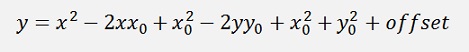
To find the minimum of the approximation the function can be written as:
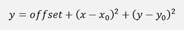
or
And the minimum is there where x – x0 = 0 and y – y0 = 0.
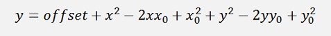
Everything a bit rearranged:
And we just computed

A parameter comparison shows that
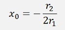
and
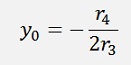
In numbers:
X0 = 2.9987
Y0 = 2.0044
And these values inserted in the above equation for z gives
Z0 = 9.0377
And that's is the minimum value of the approximated function.
The accuracy of the result is highly dependent on the quality of the input data and the learning rate and the maximum number of iteration that we allow the algorithm. Playing around with these data’s can give quite interesting results
To compute the same data in a Method of the least squares multi-dimensional brings an interesting comparison. The method of the least squares computes the approximation immediately without having to iterate. That makes the algorithm much faster and it is a bit more accurate. So, for similar problems, I would prefer the method of the least squares.
The calculation of the minimum is quite easy here as we just have a polynomial of the order 2. If the order of the polynomial is bigger, it would be a good idea to use the Newton-Maehly algorithm (see Roots of a polynomial) find the roots of this polynomial and with this the minimum of the approximation.