Method of the least squares multi-dimensional

The method of the least squares a is well known procedure to approximate a set of supporting points in the 2 dimensional spaces by a function like for instance a polynomial function (see Method of the least squares for a detailed description). But it can as well be used to approximate a multi-dimensional function to multi-dimensional supporting points.

The procedure is more or less the same as in 2 dimensional spaces. Only the setting up of the input data differs. The input data consisting of a feature vector X = (x₁, x₂, x₃,…,x_n) and a result y must be set up into an equation using a dedicated function of all input features for each factor c. So instead of

we have to set

That’s the form used on Wikipedia (looks a bit confusing). But remark: One function fi(x₁…x_n) does not necessarily have to contain all features x₁ to x_n in it.

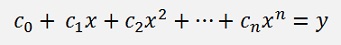
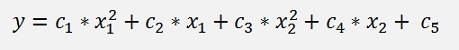
In my sample implementation I use a second degree polynomial for both of 2 input features. So my equation looks like:

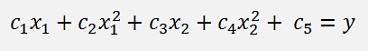
(I moved the offset c₀ to the end and changed its it to c₅)

With this equation I have to set up the input matrix equation

for my algorithm now.

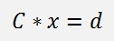
My sample data consists of 99 data sets. So I get a 99x5 matrix for C (the x and x² values) and a solution vector with 99 entries (the y values).

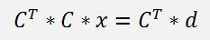
Similar to the procedure in the 2 dimensional algorithm, this matrix equation I multiplied by the transposed matrix of C like:

That reduces the 99x5 matrix equation to a 5x5 matrix equation which can be solved easily now (I use Givens rotation matrixes as they work perfect for the elimination process and I like this approach :-)

)

To have a clear algorithm, I use a separate matrix to hold the f(x) values. The data itself I keep in a class “data” that contains the collection “values” of double arrays. So the first step is to fill the matrix by the f(x) values like:

fOfX = new double[samples, features];
double[] tempD;
for (i = 0; i < samples; i++)
{
     tempD = data.values.ElementAt(i);
     fOfX[i, 0] = tempD[0];
     fOfX[i, 1] = tempD[0] * tempD[0];

     fOfX[i, 2] = tempD[1];
     fOfX[i, 3] = tempD[1] * tempD[1];
     fOfX[i, 4] = 1.0;
}

For the Givens algorithm I'm usingthe class TGivens consisting of the matrix m as a 2 dimensional double array, a solution vector y and the vector of the unknowns x is returned by the solve() function. There is a special function for multiplying this matrix by a Givens rotation matrix (this function works only for Givens rotation matrixes).

The main matrix is filled like:

for (i = 0; i < features; i++)
{
     for (j = 0; j < features; j++)
     {
         for (k = 0; k < samples; k++)
              m[j, i] = m[j, i] + fOfX[k, i] * fOfX[k, j];
     }
     for (k = 0; k < samples; k++)
     y[i] = y[i] + data.values.ElementAt(k)[2] * fOfX[k, i];
}

And with this the Givens algorithm is run (see Rotation Matrix for a detailed description):

TGivens givens = new TGivens(features, m);

givens.RunGivens();

givens.SolveRMatrix();

that yields the results for the c values of the equation

In the array givens.m.x. I used the same data I already used in Gradient descend. I use the function

That’s basically a sphere that has a radius of 4 and the centre point is at x = 3 and y=2 and the complete sphere gets an offset of 5 in z direction. But I take the square of this.

To generate the data points. Additionally I add a random value between -0.05 and +0.05

The data is stored in the data file cata.csv which is included in the project.

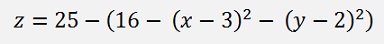
The goal is to approximate these data points and to compute the minimum of this function.

With my sample data I get the result

With these parameters the function is approximated with an average deviation of

0.001805%

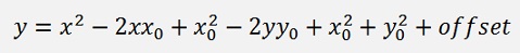
To find the minimum of the approximation the function can be written as:

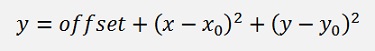
And the minimum is there where x – x₀ = 0 and y – y₀ = 0.

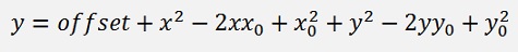
Everything a bit rearranged:

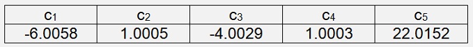
and we just computed

A parameter comparison shows that

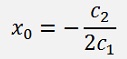
and

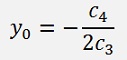
In numbers:

X₀ = 3.0012

Y₀ = 2.0009

And these values inserted in the above equation for z2 gives

Z₀ = 8.9982

which this is the minimum value of the approximated function.

Compared with the Gradient descend. using the method of the least squares is far quicker as it computes the result immediately without having to iterate and it is even a bit more accurate.

The method of the least squares has been developed by Carl Friedrich Gauss at the age of 18. That was in 1795, without a computer, without social media. Not even with electric light…unbelievable :-)

C# Method of the least squares multi-dimensional

LeastSquaresMulty.zip

Java Method of the least squares multi-dimensional

LeastSquaresMulty.zip