

I’m using a polynomial function here as I assume this is the most common way.
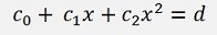
The number of unknown parameters in the searched function is lower than the number of reference points (a polynomial would have a lower order n than the number of reference points). That leads to an overdetermined system of equations. If we have for instance a set of 7 reference points (x and y) and want to approximate by a polynomial function of the 3. order, we can set up 7 equations like
The method of the least squares searches for the polynomial parameters c that lead to the smallest possible sum of the squares of the deviation of each equation.
One approach to solve this problem is the use of the normal equation.
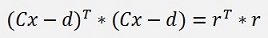
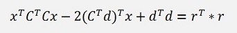
 With this conclusion that we are searching for the minimum of rT
* r
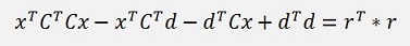
the above equation can be extended by the transposed Matrixes on both
sides and we get
With this conclusion that we are searching for the minimum of rT
* r
the above equation can be extended by the transposed Matrixes on both
sides and we get
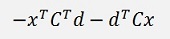
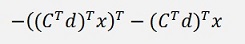 The
trick is now to realize that the whole equation for rT
* r yields just a number and not a vector nor a matrix and so these 2
terms each represent a single number too. This number can by transposed
or not, it’s the same. And so these 2 terms can be taken as
equal and we can write.
The
trick is now to realize that the whole equation for rT
* r yields just a number and not a vector nor a matrix and so these 2
terms each represent a single number too. This number can by transposed
or not, it’s the same. And so these 2 terms can be taken as
equal and we can write.
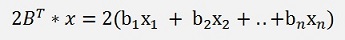
2b1
2b2
..
2bn
And that’s 2B
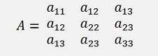
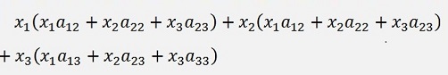
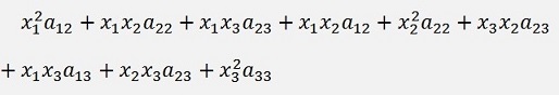
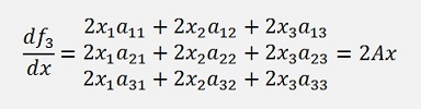
Now the third part xTAx is the most complicate and so I build it first for a 3 * 3 matrix: As A = CTC, A is symmetric to its main diagonal. So we can write

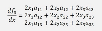
Now we put all together and get for the entire differentiation
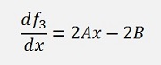
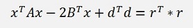
Or with the substitutions for A and B
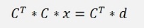
The multiplication by the transposed Matrix converts the overdetermined Matrix equation to a well determined system. In my example further above with 7 reference points and 3. Degree polynomial C has 7 lines and 3 columns. Multiplying it by its transposed makes a 3 x 3 Matrix of it and d becomes a 3 dimensional vector too. This Matrix equation can be solved by the elimination method of Gauss easily.
So the first step is to fill the Matrix equation. In C we have to put the x values of our reverence points. The first column of C consists of ones only as the first parameter we are looking for is c0 that is multiplied by 1. The second column gets x1…xn the third column (x1)2…(xn)2 and so on.
I use a 2 dimensional array as matrix m and a array for d and x. So
for (i = 0;
i <
samples; i++)
{
d[i] =
y_k[i];
for (k = 0;
k <
order; k++)
{
m[i, k]
= Math.Pow(x_k[i],
k);
}
}
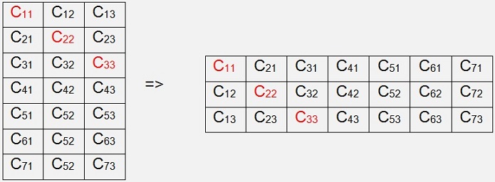
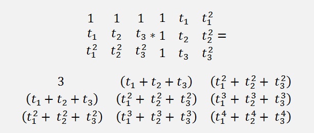
Now we have to multiply the equation by the transposed of C. The transposed Matrix of C is C mirrored at its main diagonal. In the sample the 3 x 7 Matrix becomes a 7 x 3 Matrix mirrored at the red marked main diagonal.
for (i = 0;
i <
order; i++)
{
y[i] =
0.0;
for (k = 0;
k <
samples; k++)
y[i] =
y[i] + m[k,
i] * d[k];
for (j = 0;
j <
order; j++)
{
a[j,i]
= 0.0;
for (k = 0;
k <
samples; k++)
{
a[j, i]
= a[j, i] +
m[k,j] * m[k, i];
}
}
}
Using a Cholesky decomposition to solve the matrix equation
For a detailed description of the Colesky decomposition see (see Cholesky decomposation)
Special case n = m
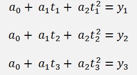
So we get the 3 equations
These do not really look like the one of the polynomial interpolation. But there is a way to see a relationship
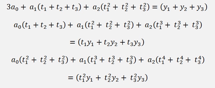
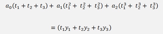
If we just add the 3 equations
Together we get

That’s already the first equation of the approximation. Now multiply the first one by t1, the second by t2 and the third by t3 and add them together. We get
That’s the second one. And finally multiply equation 1 by t12, equation 2 by t22 and equation 3 by t32 and add them all together. That makes
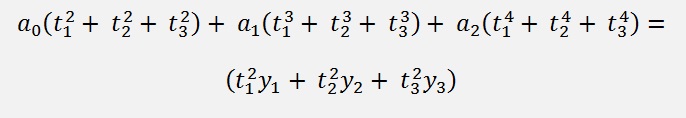
So we have all the 3 equations of the polynomial interpolation in our equations of the least squares. That means if we perform the method of the least squares in the special case of searching a polynomial of the same order as the number of supporting points we get the same parameters a0, a1, a2 as we would get them in a polynomial interpolation with the same supporting points. That means we perform a polynomial interpolation in this case.
For a n*n matrix equation it’s basically the same. Only much more calculation effort and therefore we leave that
Using orthogonal transformations
Using orthogonal transformations means basically using rotation matrixes by Givens (see RotationMatrix) and the basic idea is that the multiplication of a vector by an orthogonal matrix does not change the length of the vector and therefore the matrix equation with the residual vector
Can be transformed by these orthogonal matrixes without affecting the sum of the squares of the residua. It took me quite a while to figure out what that means. But now I think I got it
If we extend the main
matrix C which is in the sample from above a 3 * 7 matrix to get a
square matrix and set the new elements all to 0. In our sample that
looks like: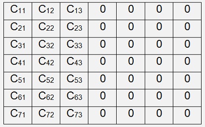
With this modified matrix the equation for the residua becomes
Now the entire equation can be multiplied by rotation matrixes to transform C’ into an upper trianglular matrix without affecting the sum of the squares of the residua. That’s an important fact.
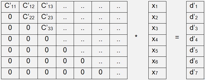
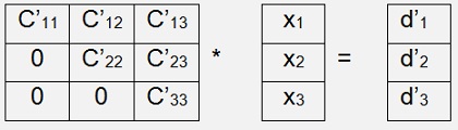
The transformation runs iterative. A rotation matrix to eliminate one certain element in C’ is built, the multiplications are carried out and then the next rotation matrix is built to eliminate the next element in C’ till we have the upper triangular matrix looking like:
public void RunGivens(int maxOrder)
{
int i, k;
for (i = 0; i < maxOrder; i++)
{
for (k = i + 1; k < maxOrder; k++)
{
if (m[k, i] != 0.0)
{
CalcRMatrix(i, k);
MultMatrix(r, i, k);
}
}
}
}
{
int i, k;
for (i = 0; i < maxOrder; i++)
{
for (k = i + 1; k < maxOrder; k++)
{
if (m[k, i] != 0.0)
{
CalcRMatrix(i, k);
MultMatrix(r, i, k);
}
}
}
}
public void CalcRMatrix(int
p, int q)
{
int i, j;
double radius;
radius = Math.Sqrt(m[p, p] * m[p, p] + m[q, p] * m[q, p]);
for (i = 0; i < m.size; i++)
{
for (j = 0; j < m.size; j++)
{
r[i, j] = 0.0;
}
r[i, i] = 1.0;
}
if (radius != 0.0)
{
if (m[p, p] == 0.0)
{
r[p, p] = 0.0;
r[p, q] = 1.0;
}
else
{
r[p, p] = m[p, p] / radius;
r[p, q] = m[q, p] / radius;
}
r[q, q] = r[p, p];
r[q, p] = -r[p, q];
}
}
{
int i, j;
double radius;
radius = Math.Sqrt(m[p, p] * m[p, p] + m[q, p] * m[q, p]);
for (i = 0; i < m.size; i++)
{
for (j = 0; j < m.size; j++)
{
r[i, j] = 0.0;
}
r[i, i] = 1.0;
}
if (radius != 0.0)
{
if (m[p, p] == 0.0)
{
r[p, p] = 0.0;
r[p, q] = 1.0;
}
else
{
r[p, p] = m[p, p] / radius;
r[p, q] = m[q, p] / radius;
}
r[q, q] = r[p, p];
r[q, p] = -r[p, q];
}
}
That builds the upper triangular matrix in r
I marked all the elements which normally are not 0 in an upper triangular matrix, but we are not interested in by “..” as these elements will become 0 in this case here anyway.
To build this upper triangular matrix we have to let p and q of the rotation matrix run from 1 to N basically. The vector d we have to multiply by the same rotation matrixes and principally r too. But as we are not really interested in r, we can leave that. Finally we have (in theory)
or
With Q as the product of all rotation matrixes. If we have a look into the transformed C now, we can see that the elements in the rows 4 to 7 are all 0. That means the elements 4 to 7 of r’ are quite fixed as element 4 to 7 of d’. We are looking for a solution of the matrix equation where the sum of the squares of the elements of r’ is the least. That’s the case when the elements 1 to 3 of r’ are 0.
That means we just have to solve this remaining matrix equation
public void Solve()
{
int k, l;
for (k = maxOrder - 1; k >= 0; k--)
{
for (l = maxOrder - 1; l >= k; l--)
{
d[k] = d[k] - x[l] * m[k, l];
}
if (m[k, k] != 0)
x[k] = d[k] / m[k, k];
else
}
{
int k, l;
for (k = maxOrder - 1; k >= 0; k--)
{
for (l = maxOrder - 1; l >= k; l--)
{
d[k] = d[k] - x[l] * m[k, l];
}
if (m[k, k] != 0)
x[k] = d[k] / m[k, k];
else
x[k]
= 0;
}}
Some speed improvement
public void RunGivens(int
maxP, int maxQ)
{
int i, k;
for (i = 0; i < maxP; i++)
{
for (k = i + 1; k < maxQ; k++)
{
if (m.c[k, i] != 0.0)
{
CalcRMatrix(i, k);
MultMatrix(r, i, k);
}
}
}
}
{
int i, k;
for (i = 0; i < maxP; i++)
{
for (k = i + 1; k < maxQ; k++)
{
if (m.c[k, i] != 0.0)
{
CalcRMatrix(i, k);
MultMatrix(r, i, k);
}
}
}
}
With maxP set to order and maxQ set to samples (see my sample project).
Compared the method of the least squares it’s a completely different approach. Isn’t that fascinating?
I implemented an online solver to do a equalisation calculus by the method of the least squares. This solver can be found here
C# Demo Projects Method of the least squares
Java Demo Projects Method of the least squares