

In the logistic regression (see Logistic Regression) the Sigmoid function
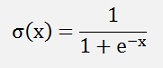
shows the tendency to saturate for very big positive or negative values of x. That’s a big disadvantage for the algorithm. But this saturation can be avoided by using the max log likelihood function as cost function for the training.
In logistic regression we have a certain amount of input data consisting of some input features x1, x2, x3,…, xn and a digital output y which has the value 0 or 1. The goal is to try to find an algorithm that can quess the correct output according to a random input x1, x2, x3,…, xn. For the derivation of the max log likelihood function we say we hypothetically have an infinite number of training samples and these samples are Bernoulli distributed. The probability mass function for an outcome y with input x1, x2, x3,…, xn is
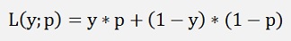
with p as the probability that the input x1, x2, x3,…, xn gives an output y = 1.In logistic regression the sigmoid function builds a probability function for the output of the regression. This probability is used in the Bernoulli mass function now with:
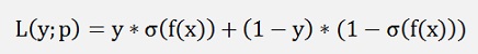
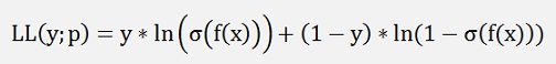
Now we want to have a as high probability to hit the correct y with the input x1, x2, x3,…, xn as possible. Therefore the output of the function L(y; p) shall be maximized. Here the logarithm comes into the scene

Calculating the logarithm of a function to be maximized changes the value of its maximum but not the position of it. So we can as well use the logarithm of p and (1-p) like:
And maximize this.
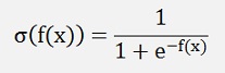
In logistic regression we have an input for the sigmoid function like
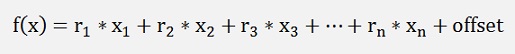
or some higher order polynomial.
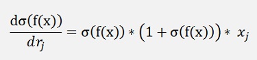
To maximize the output of LL(y;p) we have to build the gradient of LL which is the differentiation of LL with respect to r1, r2,..rn. With f(x) as a linear combination of x as above that’s:
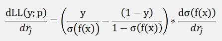
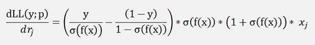
Now:
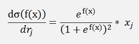
That can be written as:
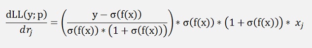
and with this
or
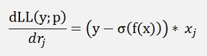
and that’s
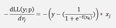
With this Gradient we compute the gradient descend now. The only thing to consider is that the maximum log likelihood looks for the maximum, but gradient descend looks for a minimum. To consider this we just take the negated of the log likelihood gradient:
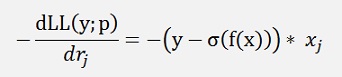
If we have a polynomial function for the input features, xj will be raised to higher power.
In my sample project for logistic regression with the Iris data set I used a polynomial of second order and had
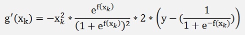
and
as the gradient.
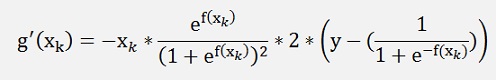
I use the same project here and just replaced this gradient by
and
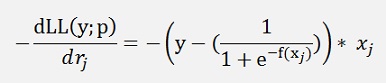
The funny thing is that, if we compare these formulations:
There is just the term
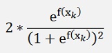
That drops out. That’s all after quite some derivation
In the update_rise function that is:
double[] update_rise(Collection<double[]> values, double[] rise, double learning_rate)
{
int i, j;
double[] d_rise = new double[features_out];
double[] x;
double y;
double e;
double[] tempSum = new double[2];
double tempValue;
for (i = 0; i < features_in; i++)
{
d_rise[2 * i] = 0;
d_rise[2 * i + 1] = 0;
tempSum[0] = 0;
tempSum[1] = 0;
for (j = 0; j < samples; j++)
{
x = values.ElementAt(j);
y = x[features_in];
e = Math.Exp(F_x(x, rise, offset));
// tempValue = 2.0 * x[i] * e / (1.0 + e) / (1.0 + e) * (y - 1.0 / (1.0 + 1 / e));
tempValue = x[i] * (y - 1.0 / (1.0 + 1 / e));
tempSum[0] = tempSum[0] - x[i] * tempValue;
tempSum[1] = tempSum[1] - tempValue;
if (Math.Abs(tempSum[0]) > 1e6)
{
d_rise[2*i] = d_rise[2*i] + tempSum[0] / samples;
tempSum[0] = 0;
}
if (Math.Abs(tempSum[1]) > 1e6)
{
d_rise[2*i+1] = d_rise[2*i+1] + tempSum[1] / samples;
tempSum[1] = 0;
}
}
d_rise[2 * i] = d_rise[2 * i] + tempSum[0] / samples;
d_rise[2 * i+1] = d_rise[2 * i+1] + tempSum[1] / samples;
}
for (i = 0; i < features_out; i++)
{
rise[i] = rise[i] - learning_rate * d_rise[i];
}
return rise;
}
With this small modification the logistic regression is carried out with maximum log likelihood instead of mean square deviation as cost function and I get to following parameters:
Iris Versicolor
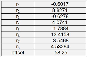
With a cost of 0.0095
Iris Setosa
With a cost of 0.00075
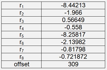
Iris Virginica
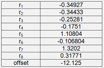
With a cost of 0.0087For the cost I still use mean square deviation here for comparision. Compared to the Logistic Regression there is no significant difference regarding the achieved cost. But if these parameters are used in the test application using the same 15 samples as in Logistic Regression the improvement becomes obvious:
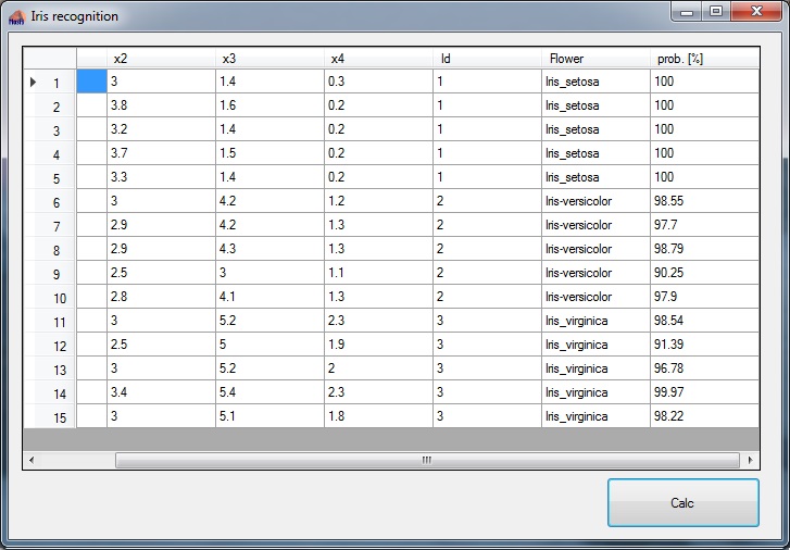
The plants are recognised with a probability of 90.25 % to 100 %. That’s quite a bit better than 52.76 % to 96.56 % with least square deviation. A remarkable improvement