

Cubic splines are a very powerful way to interpolate a curve between data points. When I implemented my first algorithm for natural cubic splines, I was quite excited how brilliant the math behind this algorithm is. The idea to implement an algorithm to draws a spline curve which adapts to a line with a random slope came to me quite soon. But it took me quite a while to figure out how to do that. O.k. meanwhile I found out and I even know that they are called “end slope splines” in the literature.
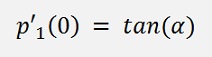
End Slope splines are defined as splines that start with a given slope on one side and end with another given slope on the other side.
The derivation of end slope splines is based on the same polynomial as natural splines are based on (see natural splines)

And they obey to the same clauses:
and
That leads to a slightly different matrix equation for ci. The matrix will get one more row and column as we have to compute c1 now and the equation line 1 and line n will be different from the others.
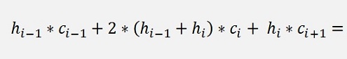
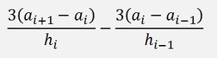
For line 2 to line n-1 the equation remains the same as it is for natural cubic splines (and its derivation is the same)
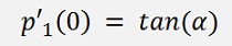
For the first line we have the clause:
and from the derivation of the natural splines we know:
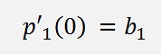
and
and so
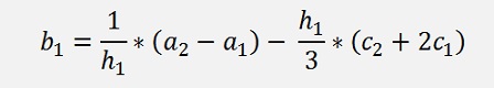
These 2 equations combined:
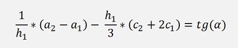
and a bit sorted:
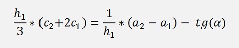
This is the equation for the first line of our matrix equation.
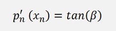
Now the last line is a bit more complicate.
Here we have
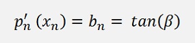
and as
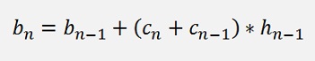
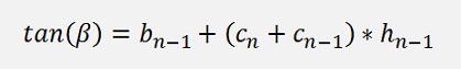
Now we use the formulation for bn-1 (from the natural cubic splines):
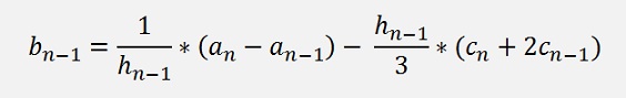
to replace bn-1 and get:
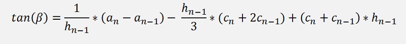
And this sorted for ci is:
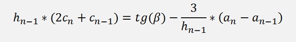
We get the formula for the last row.
With this the matrix of the matrix equation looks like:
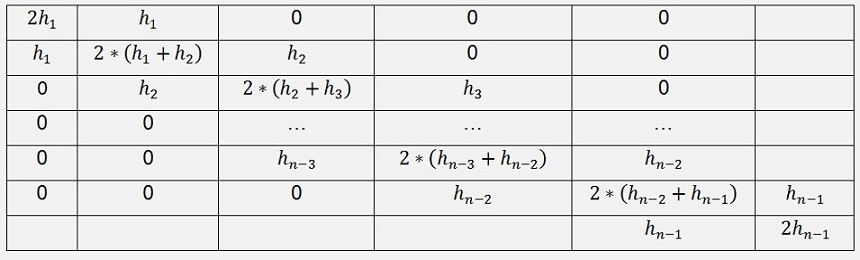
With the solution vector
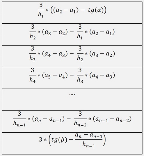
The solution of this matrix equation yields c1…cn.
With ai = yi (of the supporting points) and hi-1 = xi – xi-1.
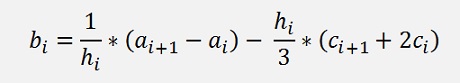
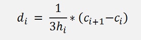
Now bi and di can be obtained by (same as with the natural cubic splines)
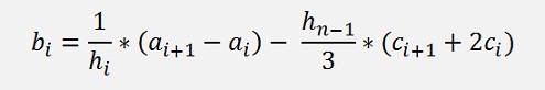
and
The C# function to this looks like:
public bool CalcParameters()
{
int i, k;
for (i = 0; i < order; i++) // calculate a parameters
{
for (i = 0; i < order - 1; i++)
{
// fill matrix for c parameters
m[0, 0] = 2.0 * h[0];
m[0, 1] = h[0];
y[0] = 3 *((a[1] - a[0]) / h[0] - Math.Tan(alpha * Math.PI / 180));
for (i = 0; i < order - 2; i++)
{
m[order - 1, order - 2] = h[order - 2];
m[order - 1, order - 1] = 2.0 * h[order - 2];
y[order - 1] = 3.0 * (Math.Tan(beta * Math.PI / 180) - (a[order - 1] - a[order - 2]) / h[order - 2]);
if (gauss.Eliminate())
{
else
return false;
}for (i = 0; i < order; i++) // calculate a parameters
{
a[i] = y_k[i];
}for (i = 0; i < order - 1; i++)
{
h[i] = x_k[i + 1] - x_k[i];
}// fill matrix for c parameters
m[0, 0] = 2.0 * h[0];
m[0, 1] = h[0];
y[0] = 3 *((a[1] - a[0]) / h[0] - Math.Tan(alpha * Math.PI / 180));
for (i = 0; i < order - 2; i++)
{
m[i + 1, i] = h[i];
m[i + 1, i + 1] = 2.0 * (h[i] + h[i + 1]);
if (i < order - 2)
m[i + 1, i + 2] = h[i + 1];
if ((h[i] != 0.0) && (h[i + 1] != 0.0))
y[i+1] = ((a[i + 2] - a[i + 1]) / h[i + 1] - (a[i + 1] - a[i]) / h[i]) * 3.0;
else
y[i+1] = 0.0;
}m[i + 1, i + 1] = 2.0 * (h[i] + h[i + 1]);
if (i < order - 2)
m[i + 1, i + 2] = h[i + 1];
if ((h[i] != 0.0) && (h[i + 1] != 0.0))
y[i+1] = ((a[i + 2] - a[i + 1]) / h[i + 1] - (a[i + 1] - a[i]) / h[i]) * 3.0;
else
y[i+1] = 0.0;
m[order - 1, order - 2] = h[order - 2];
m[order - 1, order - 1] = 2.0 * h[order - 2];
y[order - 1] = 3.0 * (Math.Tan(beta * Math.PI / 180) - (a[order - 1] - a[order - 2]) / h[order - 2]);
if (gauss.Eliminate())
{
x = gauss.Solve();
for (i = 0; i < order; i++)
{
for (i = 0; i < order ; i++) // calculate b and d parameters
{
return true;
}for (i = 0; i < order; i++)
{
c[i] = x[i];
}for (i = 0; i < order ; i++) // calculate b and d parameters
{
if (h[i] != 0.0)
{
}{
d[i] = 1.0 / 3.0 / h[i] * (c[i + 1] - c[i]);
b[i] = 1.0 / h[i] * (a[i + 1] - a[i]) - h[i] / 3.0 * (c[i + 1] + 2 * c[i]);
}b[i] = 1.0 / h[i] * (a[i + 1] - a[i]) - h[i] / 3.0 * (c[i + 1] + 2 * c[i]);
return true;
else
return false;
This function puts the spline polynomial parameters into the arrays a,b,c and d. From there the interpolated curve can be computed like:
public void Interpolate(int order, int resolution)
{
int i, k;
double timestamp;
for (i = 0; i < order - 1; i++)
{
}double timestamp;
for (i = 0; i < order - 1; i++)
{
for (k = 0; k < resolution; k++)
{
}{
timestamp = (double)(k) / (double)(resolution) * h[i];
yp[i * resolution + k] = a[i] + b[i] * (timestamp) + c[i] * Math.Pow(timestamp, 2) + d[i] * Math.Pow(timestamp, 3);
xp[i * resolution + k] = timestamp + x_k[i];
}yp[i * resolution + k] = a[i] + b[i] * (timestamp) + c[i] * Math.Pow(timestamp, 2) + d[i] * Math.Pow(timestamp, 3);
xp[i * resolution + k] = timestamp + x_k[i];
This function computes the x and y coordinates for each segment with resolution points. In me sample project I use the data points

With the angle α = 45° on the left and β = -20° on the right side the interpolated graph looks like:
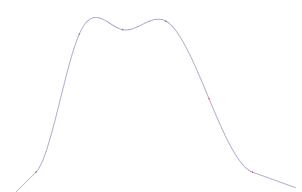
Now, this implementation as a small disadvantage: It only works for angles between -90° and 90°. That’s not too cool, but that can be avoided.
For angles from 0° to 360° the interpolation must be carried out separately for the x and the y coordinates. Therefore an additional parameter (I call it a time stamp) like t must be introduced and the interpolation must be done for y(t) and x(t) separately.
Therefore 2 sets of polynomials must be implemented and all the parameter calculation must be done 2 times.
And afterwards in the interpolation the x and y values are brought together again.
Now, there is another point to consider: For the slope we cannot use tan(α) or tan(β) anymore. That would still not work. But the solution is quite simple: We just use sin(..) for the x(t) part and cos(..) for the y(t) part. That works almost fine. The only problem is, that sinus and cosine both are limited to -1 to +1 and that’s (compared to +∞ -∞ od tan(..)) rather small I found. If we just have a look on y(t), the interpolated curve would go on with the slope that is given by the cosine of a certain angle. This slope is not too steep. The same is for the x(t) part. But when both curves are interpolated together this effect would be balanced and the slope should be correct. But it is not because the accuracy is quite bad. To avoid this I just multiplied both the sinus and the cosine value by 5. That makes the slope of both curves much steeper and therefore the resolution of the interpolation much better. And with this small modification the algorithm works quite fine

In my sample project I introduced the array t_k for the time stamps and the arrays ay, by, cy,dy for the y(t) part and ax, bx,cx and dx for the x(t) part.
The sample values I set to:
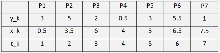
And the angles α = 30° and β = -90°.
With this the interpolated curve looks like:
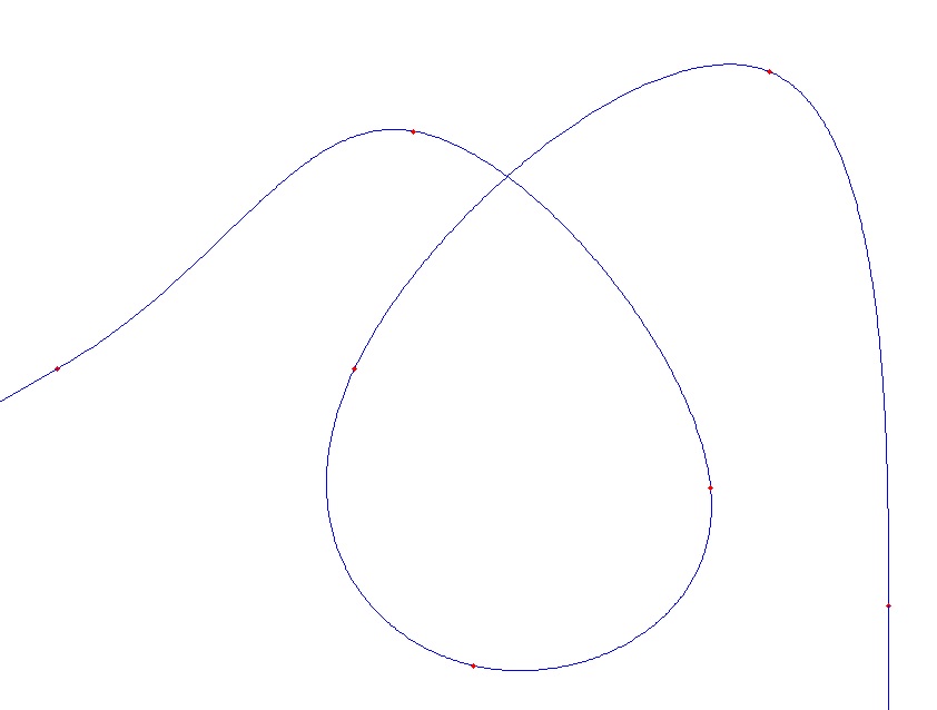
Looks quite cool..a real computer loop
For Natural splines see natural splines
For Periodic splines see periodic splines