Periodic splines
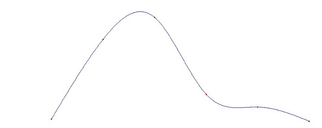
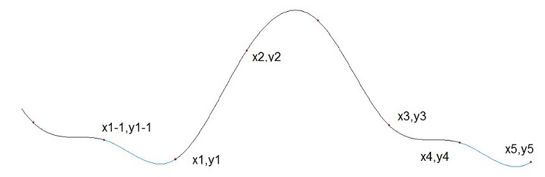
Periodic splines are meant to
interpolate a function which is periodic to the interval between the
first and the last supporting point. If we have for instance a set of 6
supporting points, the interpolation would look like this:
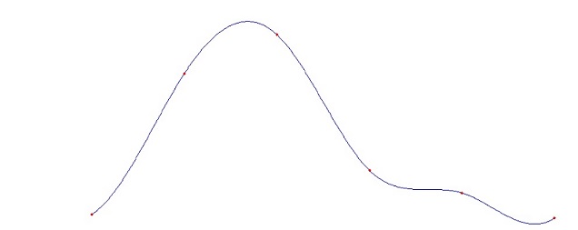
Whereas the spline function built
by natural splines with the same supporting points would look like this
There is a small difference between
these two graphs: On the periodic spline function the slope and
function value at the end and the slope and function value at the
beginning are equal. That means we could take the graph and copy and
paste it at the end of the original graph without getting a jump or
kink at the joint. On the natural splines that’s not
possible. With periodic splines we interpolate a periodic function.
The mathematical base for periodic splines is the same as the one for
natural
splines
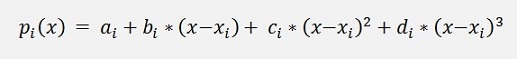
. We have the same resulting function here too:
And there are the same conditions
to be fulfilled:
a) The graph of
the functions shall meet all the supporting points
pi
(xi ) = yi
for i = 1 to n-1
b) The graph
shall not have a jump discontinuity at the supporting points
pi
(xi ) = pi-1 (xi
) for i = 2 to n-1
c) There shouldn’t be any break-points at the
supporting points
p'i
(xi ) =
p'i-1 (xi ) for i = 2 to
n-1
d) The bending of the graph shall be the same on both sides
of the supporting points
p''i
(xi ) =
p''i-1 (xi ) for i = 2 to
n-1
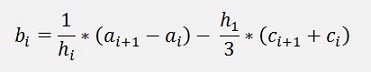
Same as for the natural spline we get from condition b
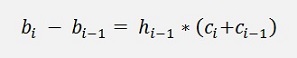
And c yields:
But now there are some additional
conditions to be fulfilled:
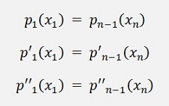
As the resulting function shall be one interval of a periodic function
it should have the same slope and the same shape at the first and the
last supporting point. That’s:
That means the conditions for the
natural splines that were valid for I = 2 to n-1 are valid for I = 2 to
n now and we have to extend the matrix equation to calculate the c
parameters by one row and one column.
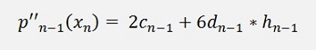
Another point is that
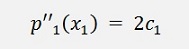
and
That shows c1
<> 0 for periodic splines and we have to calculate it.
But c1 does not appear in the matrix equation.
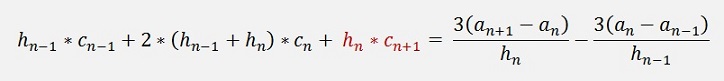
The equation for the ci parameters is the same as we already got it for
the natural splines
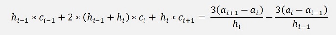
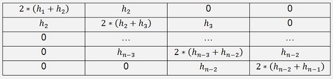
This equation led us to the
following matrix equation for natural splines:
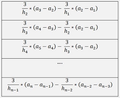
Whit the solution vector
This matrix equation we have to
extend by one row and one column for the periodic splines. With this
extension we get cn in the last column. But cn
is not on the in the
scope of the spline functions. That wouldn’t help us. The
solution is the periodicity. As our spline function should interpolate
a periodic function and a next period starts right on the right side of
the last supporting point of our graph.
we can say cn
is the same as c1. We calculate cn in the matrix
equation and use it for c1 finally. If we have a
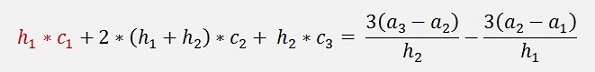
look at the equation
for the first line of the matrix equation:
c1 is
already included. We just set it to 0 for natural splines. And as it
was 0 anyway, we didn’t care that it didn’t appear
in the matrix. Now it’s not 0 anymore but it still does not
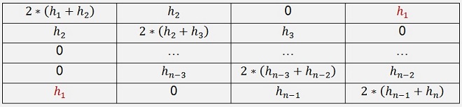
appear in the matrix. But we can write
And cn
appears in the matrix.
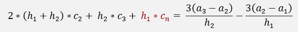
Our matrix equation has the order n -1 now and runs from 2 to n now.
The last row has the equation
Here we have the term cn+1
which
is the same as c2 and we can write
Whit this and the fact that hn
=
h1 the matrix equation becomes like
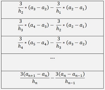
the solution vector remains almost
the same
For the solution vector is an
= a1 and an+1 = a2.
Now we can calculate all parameters. After solving the matrix equation
we just have to set c1 = cn.
An important point to consider is that we interpolate a period of a
periodic function. That means the starting point and the end point must
have the same y-value.
See Spline_periodic.zip
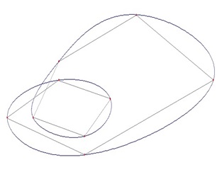
Closed loops
As a closed loop can be regarded
as a periodic function, it can be interpolated by periodic splines.
That’s quite cool 
The only thing that has to be done
is. We have to insert a kind of time stamp t to the x,y points and
interpolate the x,t sequence and the y,t separate and put them together
afterwards. To the sample sequence
I arbitrary add the time stamps
And calculate the spline
parameters for x,t and y,t. With these I build a x,y shape as a
function of t to get the above shape. This mechanism is used to draw
contour lines on maps or field lines in electrical fields
Using a Cholesky decomposition to solve the matrix equation
The Cholesky decomposition is a
quite lean approach to solve a matrix equation with some boundary
conditions. The main matrix must be symmetrical to its main diagonal
and the elements of the main matrix must be positive and bigger than
the square of the other elements in the same row. That’s the
case here and so the Cholesky decomposition can be used to solve the
matrix equation.
For a detailed description of the Colesky decomposition see (see
Cholesky decomposation)
For Natural splines see natural splines
For End slope splines see end slope splines
C# Demo Project to periodic splines
and xy function interpolating whit periodic splines
Spline_periodic.zip
Spline_XY.zip
Spline_XY_Cholesky.zip
Java Demo Project to periodic splines
and xy function interpolating whit periodic splines
SplinePeriodic.zip
SplinePeriodicXY.zip