

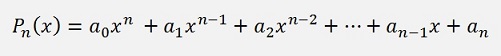
Basically

There can be an easier approach if the numbers in the polynomial are not complex but real. That’s quite often the case if an electronic filter shall be calculated and therefore a Laplace transformation of a transfer function shall be carried out.
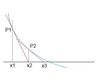
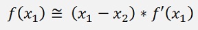
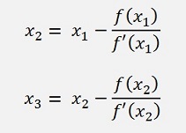
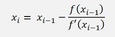
The basic procedure is the same as Newton Maehly’s algorithm. We start a certain point and run down the function till it crosses the cero line and the equation for this is still
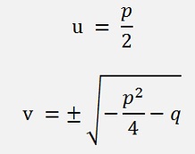
The complex root x – (u + jv) multiplied by its conjugate counterpart x - (u – jv) becomes
With a little substitution this can be written as
The next step is almost same as in the Newton Maehly algorithm: The original polynomial


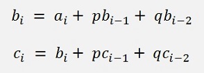
a0 = b0
a1 = b1 – p*b0
a2 = b2 – p*b1 – q*b0
…,
ai = bi – p*bi-1 – q*bi-2
This solved for b gives an algorithm to calculate the b parameters in a iterative loop:
b0 = a0
b1 = a1 + p*b0
b2 = a2 + p*b1 + q*b0
…
bj = aj + p*bj-1 + q*bj-2 for j = 2,3,...,n
Like this the b parameters can be calculated.
Now x2 – px – q is a divider of Pn(x) if bn-1 and bn both are 0.
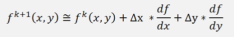
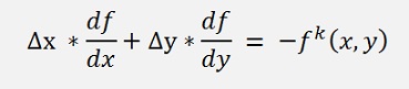
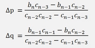
The equations for the parameters bn-1 and bn can be regarded as two independent functions and the roots of both can be found in a similar iterative function as it is done in the Newton Maehly algorithm. Only it has to be a 2 dimensional algorithm. Therefore a linearization is carried out to get an approximation for the iterations:
If the Δx and Δy of a function f(x, y) is small, the function value f(x + Δx, y + Δy) can be approximated by:
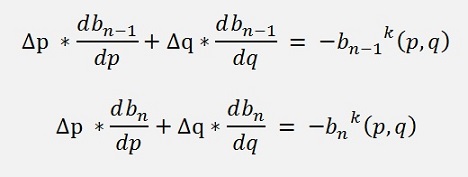
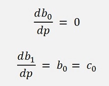
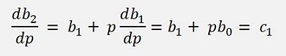
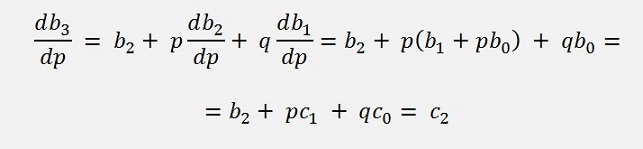
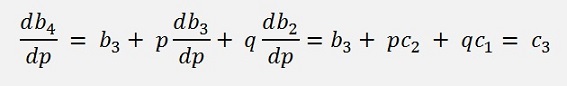
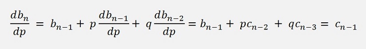
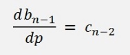
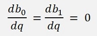
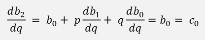
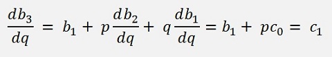
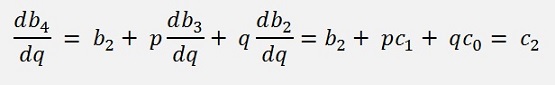
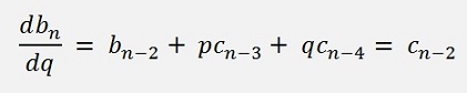
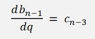
All we need now is d bn-1/dp, d bn-1/dq, d bn /dp and d bn /dq. Therefor we go back to the formulation
build the derivative of this in iterations and do some substitutions:
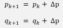
Now we have all the parts to solve the equations from above and to determine Δp and Δq: With the method of Cramer (see determinant)
and with these Δp and Δq we get the next pk+1 and qk+1 for the next iteration like:
These are all the components in theory. Now let’s put that into code.
First we build a loop to determine the values for bn, bn-1, bn-2, cn-1, cn-2 and cn-3 according to the sequence from above:
The following loop can be implemented:
bn2 = a[0];
cn2 = bn2;
bn1 = a[1] + xp * bn2;
cn1 = bn1 + xp * cn2;
cn = 0;
bn = 0;
for (i = 2; i < order; i++)
{
bn = xp * bn1 + xq * bn2 + a[i];
if (i < order - 1)
{
cn = xp * cn1 + xq * cn2 + bn;
if (i < order - 2)
{
cn2 = cn1;
cn1 = cn;
}
bn2 = bn1;
bn1 = bn;
}
}
I use bn = bn, bn1 = bn-1, bn2 = bn-2, cn = cn-1…
With these values the next p and q can be calculated as:
p = p + (bn * cn2 - bn1 * cn1) / (cn1 * cn1 - cn * cn2);
q = q + (bn1* cn - bn*cn1) / (cn1 * cn1 - cn * cn2);
But we have to make sure the divider is not 0. In this case the matrix equation would not be solvable.
I take the delta from one iteration to the next as
dxp = p - xp_old;
dxq = q - xq_old;
and put all this into a while loop checking
while ((Math.Abs(dxp)
> 1E-10) && (Math.Abs(dxq)
>
1E-10))
At the end of this loop we get p and q of x2 – px – q. This we have to decompose into
A parameter comparison shows:
That’s the complex case.
With this the algorithm finds all kinds of paired roots: Complex and real roots. In case of real roots it’s enough to compute the roots of the polynomial
And that’s
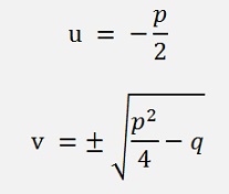
and the roots are u + v and u-v.
(see how to solve a quadratic equation)
Next step
After one pair of roots has been found, we should not stop and be happy. There could be more than one pair them
So we need to go on searching. Therefore we have to divide the original polynomial by x2 – px – q and start the same procedure again. This we repeat till the remaining polynomial is shorter or as long as x2 – px – q. Then we are finally done.
If the remaining polynomial is exactly x2 – px – q. We don’t have to search for its roots but can directly solve the quadratic equation to get the last 2 roots.
Annotation
When I was implementing this algorithm, an interesting point was that there seems no exit criteria to be needed in the loops as it is in the Newton Maehly algorithm. Bairstow always finds something and goes on searching till the polynomial is deflated enough. That’s quite nice and makes live uncomplicated
In my sample project I use the function FindRoot(…) to find one pair of real or complex roots. The parameters p and q of this pair is stored in the list
public List<SRoot>root
In a loop all paired roots are searched and stored in this list. Afterwards I run though this list, check the p and q parameter of each pair and accordingly the real and complex roots of them are extracted.
At end the remaining polynomial is displayed as well as the found roots.
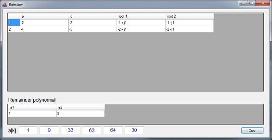
In the list box above for each paired root the parameter p and q and the found roots to them are displayed.