

Homogeneous first order differential equation
Homogeneous case sample
Inhomogeneous first order differential equation
Inhomogeneous case sample
Bernoulli differential equation
Bernoulli differential equation sample
In natural sciences and engineering sciences differential equations are very important as there are many natural laws expressed by them. A differential equation is the physical modelling of a natural phenomenon where the wanted function appears as function and its differentiation as well in one equation. The differentiation can appear in various orders (not only the first). The highest differentiation gives the order of the differential equation.
The simplest form of a differential equation is the homogeneous first order differential equation. So we start with that.
Homogeneous first order differential equation
In the homogeneous first order differential equation there is just the wanted function and its differentiation and no additional term. Its formulation is:
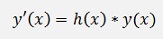
or
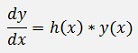
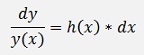
To solve this equation for the wanted function y(x) a so called variable separation is carried out. That means the equation is multiplied by dx and divided by y to get x onto the right and y onto the left side:
Now both sides must be integrated.
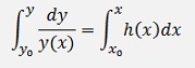
The left side is integrated with y and the right side with x. Here the initial values x0 and y0 must be taken into account.
In a first step only the integration of left side is carried out:
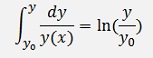
And so
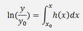
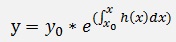
Now on both sides the exponential function is applied:
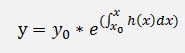
and that’s the general solution for the homogeneous first order differential equation.
Homogeneous case sample
In the sample:
There is
and
and with this
and if x0 = 0
Inhomogeneous first order differential equation
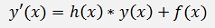
The inhomogeneous first order differential equation is more or less an extension of the homogeneous one. It has an additional term f(x) on the right side. Its formulation is:
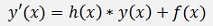
Where f(x) is called the disruptive term.
To solve this equation a so called variation of the constants is carried out.
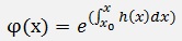
Starting from the solution for the homogeneous case
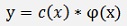
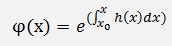
The constant y0 is replaced by a function c(x) and say
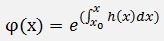
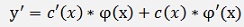
and the differentiation of φ(x) is:
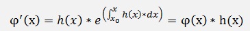
and with this φ(x) the homogeneous case becomes
and its differentiation
Or with the formulation for φ’(x) from above
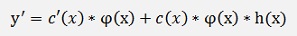
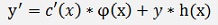
Now. As
we can replace c(x) * φ(x) by y and get
If we compare this with the equation of the inhomogeneous case
Its obvious that
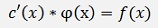
and that’s a homogeneous differential equation for c(x)
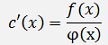
and the solution for this is
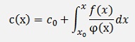
With this inserted in

the solution for the inhomogeneous case becomes
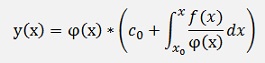
with φ(x) as we defined further above:
Where c0 = y0
If this solution is written without brackets
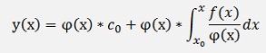
The part φ(x)* c(x) is the solution of the homogeneous case and the part on the very right is the extension to the inhomogeneous case.
Inhomogeneous case sample
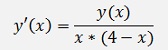
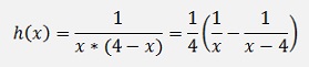
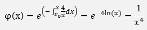
In the sample of an inhomogeneous differential equation:
There is
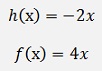
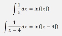
and so
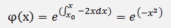
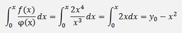
and
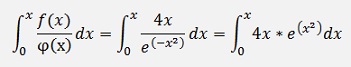
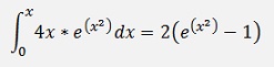
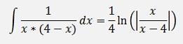
And with this
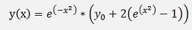
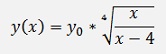
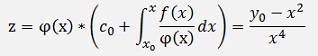
The solution

Bernoulli differential equation
A differential equation like
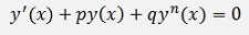
is called Bernoulli differential equation.
To solve such an equation the approach is the substitution

Where z shall be a function.
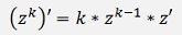
For the substitution of y’(x) the chain rule for differentiations must be applied (see Differential calculus). If z is a function f(x), zk is a chain like
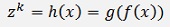
Where

and with the chain rule
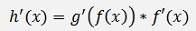
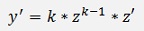
we get
And therefore
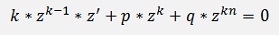
With this the equation becomes
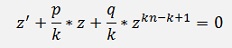
or divided by k * zk-1:
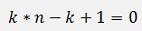
Now, if k is defined as

Then
And we get a linear inhomogeneous differential equation
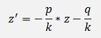
That can be solved with the approach from above with
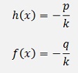
or with the n of yn
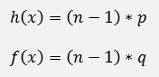
Bernoulli differential equation sample
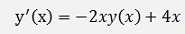
The sample
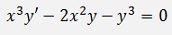
Is a Bernoulli differential equation.
To solve this, it must be brought into the form of the Bernoulli differential equation by dividing the whole equation by x3.
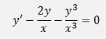
Now we have
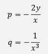
And as n = 3

With this
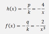
With the solution for the homogeneous case
and the inhomogeneous part
With these the solution for z becomes:
And as we made the substitution y = zk, we have to undo that to get the solution for y and get:
That’s it