

The Chebyshev polynomials are named after the Russian mathematician Pafnuty Lvovich Chebyshev. They are used in approximation and interpolation algorithms.
The interpolation by the use of Chebyshev polynomials makes the substitution x = cos(φ) and uses the basic formulation

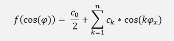
And is basically a kind of a cosine transformation. Because the cosine function returns -1 to +1, this transformation is basically defined in the interval -1 to +. But later on this limitation will vanish.
The cos(kφ) is a bit transformed.
With the addition theorem
and therefore
and with n = 1
or
Or for 2φ
and for 3φ
or
and in the same manner:
and so on...
Now there comes the substitution cos(φ) = x and cos(nφ) = Tn(x) and with this
And so on.
This sequence can be written in a recursive formulation as
That’s the recursive formulation for a Chebychev polynomial.
O.k. the approximation of given function is possibly not the most interesting thing. But it gives a good view how the Chebychev polynomials work
With the above substitution the approximation formula
becomes:
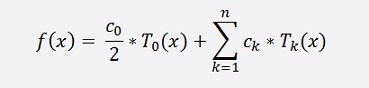
and the ck parameters are
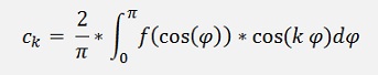
If we have a look at a Fourier transformation, ck corresponds to the ak parameter of the Fourier transformation of the even function f(cos(φ)) (See Discrete Fourier transformation).
In other words: To compute the ck parameters is to compute the Fourier parameters of f(cos(φ)).
To solve this integral is quite a complicate task. But as we just have to compute Fourier parameters, we can do this by a rather simple DFT for some supporting points of this function and that’s quite easy.
So I did the sample f(x) = x3 and made the following code to this:
private double f_x(double x)
{
return
x*x*x;
}Compute the ck parameters:
public void CalcCParams() // calculation of the Fourier parameters
{
int
k, n;
if (order > 0)
{
}if (order > 0)
{
for
(k = 0; k < order; k++)
{
c[0] = c[0] / 2.0;
}{
c[k]
= 0;
for (n = 0; n < (order); n++)
{
c[k] = c[k] / order * 2;
}for (n = 0; n < (order); n++)
{
c[k]
=
c[k] + Math.Cos(2.0
* Math.PI
* (k * n) / (double)order)
* y_k[n];
}c[k] = c[k] / order * 2;
c[0] = c[0] / 2.0;
and to approximate the curve:
public void Approximate(int maxPoints, double maxTime)
{
int
i;
for (i = 0; i <= maxPoints; i++)
{
}for (i = 0; i <= maxPoints; i++)
{
yp[i]
=
0;
xp[i] = (a + (b - a) * (double)(i) / (double)maxPoints);
yp[i] = CalcChebychev (xp[i],6);
}xp[i] = (a + (b - a) * (double)(i) / (double)maxPoints);
yp[i] = CalcChebychev (xp[i],6);
with
public double CalcChebychev(double x, int order)
{
int
i;
double[] t = new double[7];
double value;
t[0] = 1;
t[1] = x;
for (i = 2; i < order; i++)
for (i = 1; i < order; i++)
}double[] t = new double[7];
double value;
t[0] = 1;
t[1] = x;
for (i = 2; i < order; i++)
t[i]
= 2
* x * t[i - 1] - t[i - 2];
value
= c[0];for (i = 1; i < order; i++)
value
=
value + c[i] * t[i]; ;
return
value;All put together:
for(i = 0 ; i < order; i++)
{
x_k[i] = (double)(i) / (double)order;
y_k[i] = f_x(Math.Cos(x_k[i] * Math.PI * 2.0 ));
}
CalcCParams();
Approximate(datapoints, b);
After this sequence the approximated curve is in the arrays xp and yp and can be drawn into a graph
The advantage of the Chebychev polynomials is that by the cosine transformation the coordinate system becomes a bit deformed. It will be compressed close to the outer limits. So the function values at the outer limits (closer to +π/2 and –π/2) get closer to each other than the ones close to the center (close to 0). If there were supporting points at equal shift, that would be like:
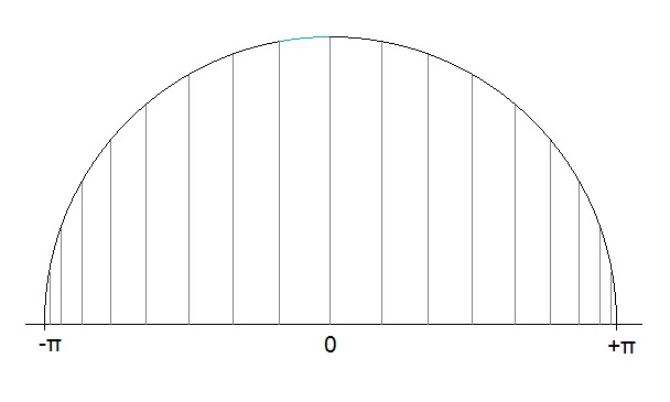
The supporting points would be spread on a circle with the same segment of the circle between them (the blue segment).
The interesting point of this is, that the inaccuracy of the approximation is more influenced by the distance between the supporting points at the outer limits than the ones near the center and due to this fact, using Chebychev polynomials for an approximation yields a smaller inaccuracy than other algorithms.
O.k. to approximate a known function is probably not that interesting. But it’s good to see how Chebychev polynomials work and that’s good to know if it comes to an interpolation by the use of Chebychev polynomials
The interpolation of a unknown function with just some supporting points is much more interesting than to approximate a given function.
The approach is a bit different from above. Here the ck parameters cannot be computet straight forward. But the formulation
Leads to a matrix equation like for instance:
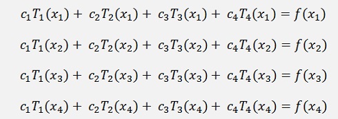
for 4 supporting points.
In this matrix equation the ck parameters are the unknowns and Tk(xi) are Chebychev polynomials that must be computed for each xi. To compute the ck parameters we have to set up this matrix equation and solve it by, for instance, the Gaussian elimination algorithm.
Therefore I changed the function CalcChebychev a bit:
public
double
CalcChebychev(double
x, int order)
{
int i;
double value;
t[0] = 1;
t[1] = x;
for (i = 2; i < order; i++)
t[i] = 2 * x * t[i - 1] - t[i - 2];
t[0] = 0.5;
value = c[0]/2.0;
for (i = 1; i < order; i++)
value = value + c[i] * t[i];
return value;
}
{
int i;
double value;
t[0] = 1;
t[1] = x;
for (i = 2; i < order; i++)
t[i] = 2 * x * t[i - 1] - t[i - 2];
t[0] = 0.5;
value = c[0]/2.0;
for (i = 1; i < order; i++)
value = value + c[i] * t[i];
return value;
}
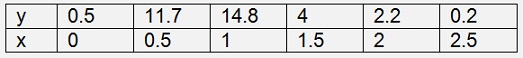
The supporting points to be interpolated I put into x_k and y_k and fill the matrix equation upside down to increase the accuracy of the elimination algorithm like:
for
(i = 0; i < order; i++)
{
CalcChebychev(x_k[order - 1 - i], order);
m.y[i] = y_k[order - 1 - i];
for (k = 0; k < order; k++)
{
m.a[i, k] = t[k];
}
}
{
CalcChebychev(x_k[order - 1 - i], order);
m.y[i] = y_k[order - 1 - i];
for (k = 0; k < order; k++)
{
m.a[i, k] = t[k];
}
}
if
(gauss.Eliminate())
{
{
gauss.Solve();
for (i = 0; i < order; i++)
c[i] = m.x[i];
Interpolate(datapoints, x_k[0], x_k[order - 1]);
}for (i = 0; i < order; i++)
c[i] = m.x[i];
Interpolate(datapoints, x_k[0], x_k[order - 1]);
public
void Interpolate(int
maxPoints, double
minTime, double
maxTime)
{
{
int
i;
for (i = 0; i < maxPoints; i++)
{
}for (i = 0; i < maxPoints; i++)
{
yp[i]
=
0;
xp[i] = (double)(i) * (maxTime - minTime) / (double)maxPoints;
yp[i] = CalcChebychev(xp[i], order);
}xp[i] = (double)(i) * (maxTime - minTime) / (double)maxPoints;
yp[i] = CalcChebychev(xp[i], order);
(For the class gauss see The elimination algorithm by Gauss).
My sample shape for the supporting points.
Creates the following output:
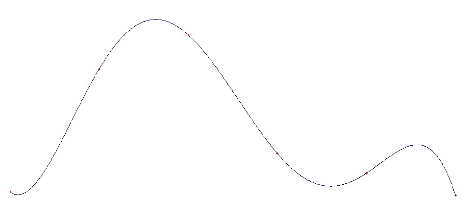
And interestingly the limits of -1 to +1 for x are gone and the cosine to
C# Demo Projects to Chebychev polynomials