

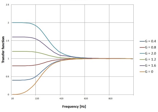
Digital filters like the Bessel, Butterworth or Chebychev filter cut down the output signal to 0 in the blocking band. This is not always wanted. In digital equalizing for instance we just want to reduce or boost the output signal by a certain amount in the blocking band. This can be done by the Shelving filter. The shelving filter uses an amplification factor G that increases the output signal if bigger than 1 or decreases it if smaller than 1.
Drawing the transfer function for different values of G gives the specific image that gives the filter its name:
It looks like (with some fantasy
 ) a continental shelf
(https://en.wikipedia.org/wiki/Continental_shelf).
In the German
speaking areas it’s even better. There they call
“Kuhschwanz Filter”,
(https://de.wikipedia.org/wiki/Kuhschwanzfilter)
what means exactly
translated "cow tail filter", because the transfer function would look
like a
waving cow tail. I think they have no idea about cows.
) a continental shelf
(https://en.wikipedia.org/wiki/Continental_shelf).
In the German
speaking areas it’s even better. There they call
“Kuhschwanz Filter”,
(https://de.wikipedia.org/wiki/Kuhschwanzfilter)
what means exactly
translated "cow tail filter", because the transfer function would look
like a
waving cow tail. I think they have no idea about cows.
Cows are so lovely beings
Cows don’t care for digital filtering
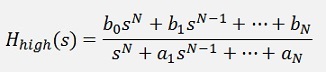
As the Shelving filter uses an amplification factor which can be bigger or smaller than 1, it is not that easy to distinguish a high pass from a low pass filter. Usually a high pass filter affects the low frequencies of a signal and leave the high frequency’s untouched. The same is here: At the high pass Shelving filter the transfer ration at high frequency’s is 1.
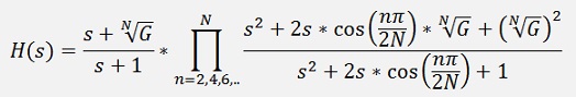
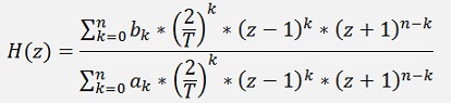
The transfer ration for lower frequencies depends on the amplification G.The transfer function of the Shelving filter in the Laplace domain is:
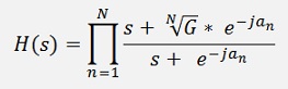
with
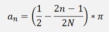
and G as the amplification.
On the first glimpse that looks quite strange. Complex numbers in the s domain are rather unusual. But if we spend the effort and do some calculations, we get for
N = 2
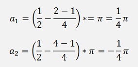
and the enumerator
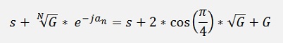
and denominator
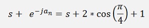
the transfer function becomes:
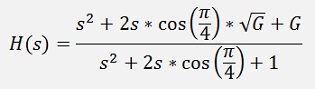
which is similar to
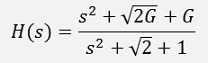
As it is usually written in the literature.
(See Complex numbers for the math with complex numbers)
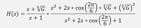
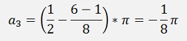
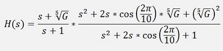
For N = 3:
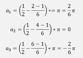
And, similar to above, the transfer function becomes:
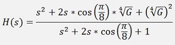
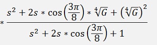
For N = 4
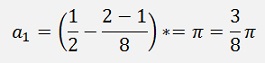
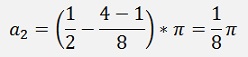
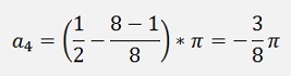
The transfer function becomes a bit bigger
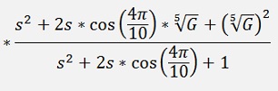
And for N = 5
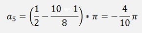
A kind of an order becomes visible for the transfer function:
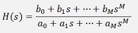
These transfer functions can be written in general formulations:
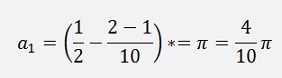
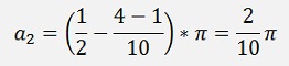
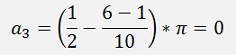
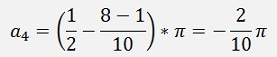
For N is even we get:
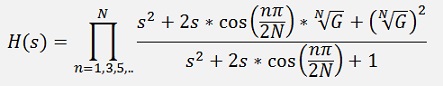
Only odd n’s.
For N is odd we get:
Only even n’s.
And that’s quite easy to be implemented in a C# function:
public void CalcShelving(double amp)
{
int i = 1;
a_s = new double[1];
b_s = new double[1];
double[] poly = new double[3];
double gl = Math.Pow(amp, 1.0 / order);
double tempD;
if (order % 2 == 0) // order is even
{
a_s = new double[1];
b_s = new double[1];
b_s[0] = 1.0;
a_s[0] = 1.0;
for (i = 1; i < order; i += 2)
{
poly[0] = 1.0;
poly[1] = 2.0 * Math.Cos(Math.PI * i / 2.0 / order) * gl;
poly[2] = gl * gl;
b_s = Poly.Mult(b_s, poly);
poly[0] = 1.0;
poly[1] = 2.0 * Math.Cos(Math.PI * i / 2.0 / order);
poly[2] = 1.0;
a_s = Poly.Mult(a_s, poly);
}
}
else // order is odd
{
a_s = new double[2];
b_s = new double[2];
b_s[0] = 1.0;
b_s[1] = gl;
a_s[0] = 1.0;
a_s[1] = 1.0;
for (i = 2; i < order; i += 2)
{
poly[0] = 1.0;
poly[1] = 2.0 * Math.Cos(Math.PI * i / 2.0 / order) * gl;
poly[2] = gl * gl;
b_s = Poly.Mult(b_s, poly);
poly[0] = 1.0;
poly[1] = 2.0 * Math.Cos(Math.PI * i / 2.0 / order);
poly[2] = 1.0;
a_s = Poly.Mult(a_s, poly);
}
}
for (i = 0; i < b_s.Length / 2; i++)
{
tempD = b_s[i];
b_s[i] = b_s[b_s.Length - 1 - i];
b_s[a_s.Length - 1 - i] = tempD;
}
}
The class Poly is a small static class for polynomial math I implemented.
This function returns the transfer function in the s domain in the arrays a_s and b_s. With a_s[0] as the first parameter a0 in the polynomial.
This transfer function must be converted into the transfer function in the z domain which is done by the bilinear transformation (see Digital filter design):
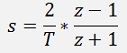
with
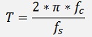
and fc = cut off frequency of the filter and fs = sampling frequency. If this transformation is done and the compound fractions are removed we get.
For this transformation I use more or less the same function I already used in Butterworth filter:
public void TransformToZPlane()
{
int i, j;
List<double[]> aa = new List<double[]>();
List<double[]> bb = new List<double[]>();
double[] tempA = { 1.0, 1.0 };
tempA[0] = 1;
tempA[1] = 1;
for (i = 0; i < a_s.Length; i++)
{
aa.Add(new double[] { 1.0, -1.0 });
bb.Add(new double[] { 1.0, -1.0 });
}
for (i = 0; i < a_s.Length; i++)
{
double[] tempEl = aa.ElementAt(i);
tempEl = Poly.Mult(Poly.Power(tempA, i), Poly.Power(tempEl, a_s.Length - 1 - i));
tempEl = Poly.Mult(tempEl, a_s[i] * Math.Pow(2.0 / wc, a_s.Length - 1 - i));
aa.RemoveAt(i);
aa.Insert(i, tempEl);
}
for (i = 0; i < b_s.Length; i++)
{
double[] tempEl = bb.ElementAt(i);
tempEl = Poly.Mult(Poly.Power(tempA, i), Poly.Power(tempEl, b_s.Length - 1 - i));
tempEl = Poly.Mult(tempEl, b_s[i] * Math.Pow(2.0 / wc, b_s.Length - 1 - i));
bb.RemoveAt(i);
bb.Insert(i, tempEl);
}
a_z = new double[aa.Count];
for (i = 0; i < a_z.Length; i++)
{
a_z[i] = 0;
for (j = 0; j < aa.Count; j++)
{
a_z[i] = a_z[i] + aa.ElementAt(j)[i];
}
}
b_z = new double[bb.Count];
for (i = 0; i < b_z.Length; i++)
{
b_z[i] = 0;
for (j = 0; j < bb.Count; j++)
{
b_z[i] = b_z[i] + bb.ElementAt(j)[i];
}
}
for (i = 0; i < b_z.Length; i++)
{
b_z[i] = b_z[i] / a_z[0];
}
for (i = a_z.Length - 1; i >= 0; i--)
{
a_z[i] = a_z[i] / a_z[0];
}
}
The variable wc is the T from above.
Now the transfer function in the z domain is in the arrays a_z and b_z and the Shelving filter is ready to use like:
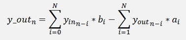
The following code fragment shows how I implemented that:
t = 2.0 * Math.PI * fc / fs;
TShelving shelv = new TShelving(order, t);
shelv.CalcShelving(G, cbHighPass.Checked == true);
shelv.TransformToZPlane();
a = shelv.a_z;
b = shelv.b_z;
// create a signal
for (i = 0; i < datapoints; i++)
{
t_in[i] = i / fs;
y_in[i] = 20.0 * Math.Sin(2.0 * Math.PI * t_in[i] * f);
}
// as long as there are not enough values to fill the polynomials
for (i = 0; i < a.Length; i++)
{
y_out[i] = 0;
for (j = 0; j <= i; j++)
{
y_out[i] = y_out[i] + y_in[i-j] * b[j];
}
for (j = 1; j <= i; j++)
{
y_out[i] = y_out[i] - y_out[i-j] * a[j];
}
}
// now there are enough values
for (i = a.Length; i < datapoints; i++)
{
y_out[i] = 0;
for (j = 0; j < a.Length; j++)
{
y_out[i] = y_out[i] + y_in[i - j] * b[j];
}
for (j = 1; j < a.Length; j++)
{
y_out[i] = y_out[i] - y_out[i - j] * a[j];
}
if ((y_out[i] > max) && (i > 100))
max = y_out[i];
}
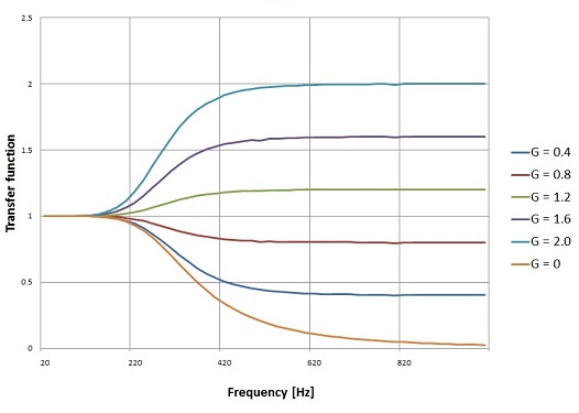
With N = 3, cut off frequency = 300 Hz and samlpling frequency = 10 kHz that creates the following transfer functions for different G’s
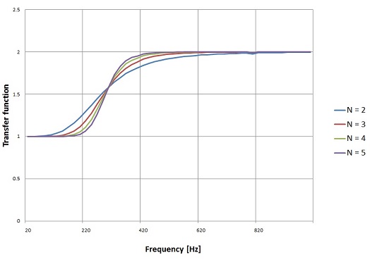
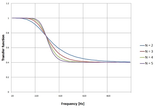
And with a fixed G = 2.0 and N = 2 to 5.
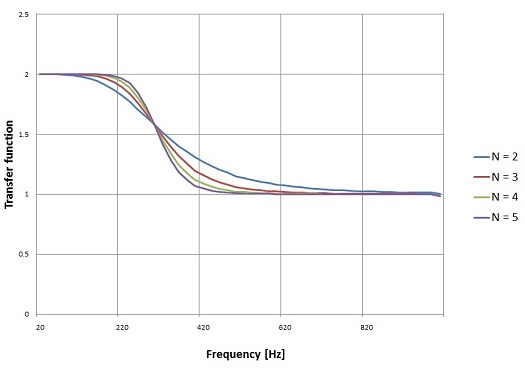
Looks possibly a bit confusing as it is a high pass filter and it increases the output at low frequencies. But high pass means the filter affects to low frequencies ant leaves the high frequencies untouched.
Or for G = 0.4:
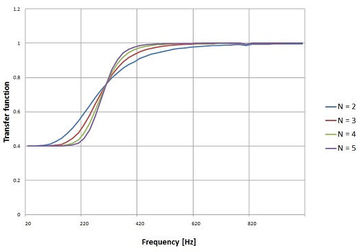
Low pass Shelving filter
To get the same functionality on the high frequency side we have to do a high pass to low pass transformation. This is done by the substitution of s by 1/s in the Laplace domain.
For a transfer function like
hat is
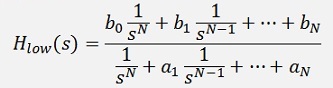
If we remove the compound fractions, that just switches the order of the ai and the bi values what can be done in the function
public void CalcShelving(double
amp, bool bHighPass)
by adding the parameter bHighPass and modifying the lines at the end of the function to:
if(!bHighPass)
{
for(i=0; i < a_s.Length / 2; i++)
{
tempD = a_s[i];
a_s[i] = a_s[a_s.Length - 1 - i];
a_s[a_s.Length - 1 - i] = tempD;
}
for (i = 0; i < b_s.Length / 2; i++)
{
tempD = b_s[i];
b_s[i] = b_s[b_s.Length - 1 - i];
b_s[a_s.Length - 1 - i] = tempD;
}
}
That’s all
With this we get the graphs:
For N = 3 and various G’s.
With fixed G = 2.0 and various N’s
With fixed G = 0.4 and various N’s.
The Shelving filter could easily be transformed into a band block filter as I did it in Digital band pass and band stop filter. But I think that does not make too much sense as this filter would have the same G on the high and low frequency side. That wouldn’t be that cool
A online solver in JavaScript, that returns the filter parameters, can be found on Shelving filter
C# Demo Project Shelving filter