

Basically
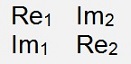
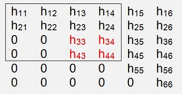
To compute real and complex Eigenvalues of a random matrix there are two steps involved: First the matrix is brought to Hessenberg form. This is done to simplify the computation of the Eigenvalues and to reduce the calculation effort later on. In a second step the Eigenvalues of this Hessenberg formed matrix are computed in an iterative loop performing a QR decomposition and RQ re-composition to approach the Eigenvalues in the main diagonal. Doing this loop repeatedly the diagonal elements should converge to the eigenvalues. At the end, if there are only real eigenvalues, all the main diagonal elements are eigenvalues. If there are conjugate complex eigenvalues, two conjugate complex eigenvalues will be held in a sub matrix of the size 2*2 as shown here in the elements h33, h34, h43 and h44.
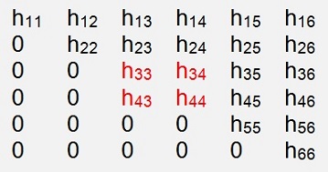
and they will be set like
I wrote they “should” converge as they do not for sure. Especially if there are conjugate complex eigenvalues. Therefore it’s better not to try to compute all eigenvalues at once but just to observe the last diagonal element (or the last 2 elements in case of complex eigenvalues) and as soon as this element or elements have converged enough, this eigenvalue is saved, the last row and last column is cut off and the QR decomposition starts with the reduced matrix again. And this procedure is repeated until all eigenvalues are found.
Transformation to Hessenberg form
A matrix in Hessenberg form looks like (here a 6*6 matrix)
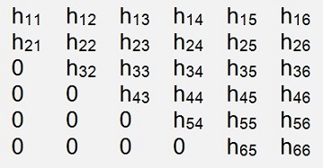
All the elements below one element below the main diagonal are zero.
The transformation is done by the use of rotation matrixes (as usual
 )
and he rotation matrix U(p, q, φ) used for these
transformations looks like:
)
and he rotation matrix U(p, q, φ) used for these
transformations looks like:
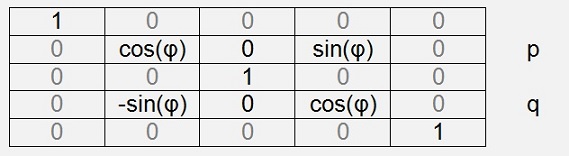
(See Rotation matrix for an introducition to rotation matrixes)
But now not the element aqp shall be eliminated by the multiplication but the element aqp-1. That is to avoid manipulating the element that has been eliminated by the preceding multiplication.
Now an important point is that there are not just elements eliminated. There shall be a similarity transformation and that means the matrix A is multiplied by the transposed rotation matrix from left first and the result of this multiplication is multiplied by the rotation matrix itself from right like
The multiplication by UT eliminates the elements and the multiplication by U makes the similarity and does not affect the eliminated elements.
So we have to determine the rotation angle first and therefore the transposed rotation matrix is used.
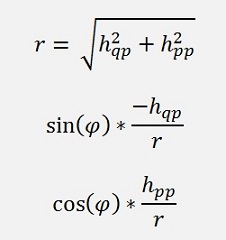
Multiplying UT by A gives for a’qp-1 which should be eliminated
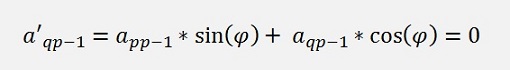
To get this equation to 0 we set
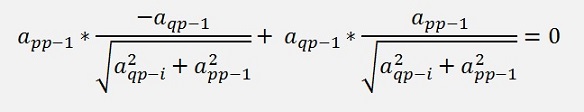
and with
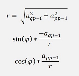
In the literature mostly the formulation looks like
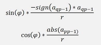
That rotates always counter clockwise. The above formulation does not. That’s all. Besides this I haven’t seen a different behaviour for these two formulations so far and so I prefer to use the simpler one
.If app-1 = 0 there is now need for calculations and we can just set sin(φ) = 0 and cos(φ) = 1
With this formulation the function to compute the rotation matrix looks like:
public void CalcRMatrixHess(int p, int q)
{
int i, j;
double radius;
radius = Math.Sqrt(m.a[p, p - 1].real * m.a[p, p - 1].real + m.a[q, p - 1].real * m.a[q, p - 1].real);
for (i = 0; i < m.size; i++)
{
for (j = 0; j < m.size; j++)
{
r.a[i, j].real = 0.0;
}
r.a[i, i].real = 1.0;
}
if (radius != 0.0)
{
if (m.a[p, p - 1].real == 0.0)
{
r.a[p, p].real = 0.0;
r.a[p, q].real = 1.0;
}
else
{
r.a[p, p].real = m.a[p, p - 1].real / radius;
r.a[p, q].real = - m.a[q, p - 1].real / radius;
}
r.a[q, q].real = r.a[p, p].real;
r.a[q, p].real = -r.a[p, q].real;
}
}
And the function to transform the matrix m into Hessenberg form:
public void RunHessenberg(int order)
{
int p, q;
for (p = 1; p < order - 1; p++)
{
for (q = p + 1; q < order; q++)
{
if (Math.Abs(m.a[q, p - 1].real) > 1E-200)
{
CalcRMatrixHess(p, q);
m.MultTranspMatrixLeft(r, p, q);
m.MultMatrixRight(r, p, q);
}
}
}
}
Now the matrix is ready to compute the eigenvalues and eigenvectors.
The second step is a bit more complicate and there is much less useful documentation to be found. It took me quite some time to find all the pieces of the puzzle to implement a working algorithm.
In a first step in most of the literature they have a look how to compute “real eigenvalues” and afterwards they go to “complex eigenvalues”. There my approach differs a bit from what is written in most articles about this topic. First there is a simply case: There are real eigenvalues in the main diagonal. Then there is a complex case with complex or real eigenvalues in a 2x2 matrix in the main diagonal and below. But more to this later.
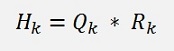
The procedure to compute eigenvalues out of this Hessenberg matrix H is to decompose the matrix H into the matrix Q and R and then doing the hole transformation backwards by multiplying R * Q in a iterative loop. That’s simple spoken.
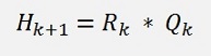
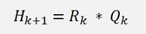
The matrix R is a upper diagonal matrix and Q is an orthogonal matrix composed of rotation matrixes. In the iterative loop we build Hk+1 out of Hk with the formulation:
and
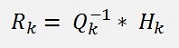
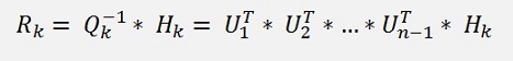
With the first formula resolved for Rk:
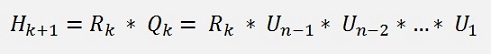
As I already mentioned: Q is composed of rotation matrixes and these we have to determine. To transform H into an upper diagonal matrix only the elements below the main diagonal have to be eliminated (as all the elements below them are 0 already in the Hessenberg matrix). For a N*N matrix that takes N-1 rotations. So we will get N-1 rotation matrixes and as Q is inverse in this formula we use inverse rotation matrixes U1-1…Un-1-1 as well. That makes it easier afterwards.
So the formulation is
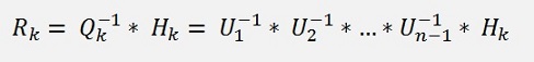
Now the big point is that the inverse of a rotation matrix is its transposed matrix. That can easy be seen if we multiply U * UT we get I (the unit matrix) and that means UT =U-1. So the above formula can be written as
And we get first a transposed rotation matrix like (only the signs of the sin switched)
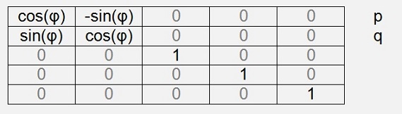
With p = 1 and q = 2 to eliminate element h’21
and get the equation
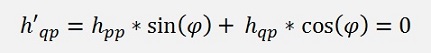
and almost similar to the formula further above
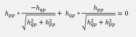
and with
This we have to do for h’21 to h’nn-1 now and multiply each of these rotation matrixes by our origin Hessenberg matrix to get the matrix R finally (and remark: As we used the transposed rotation matrix for this formulation the result for the sinus and the cosine’ will be for the not transposed matrix and it will have to be multiplied transposed for the QR transformation).
Now there comes another important point: The QR transformation together with its backward RQ transformation is a similarity transformation and so each multiplication of one transposed rotation matrix with H should build a similarity transformation with the following multiplication of R with the not transposed rotation matrix in the equation
o.k. that sounds quite complicate but I don’t know how else to explain that
Simply spoken it means:
Just remark the switched order of the U matrixes. That’s the point.
The backward transformation has to be done in inverted order. That means we have to save the angles used in the QR transformation and use them backward in the RQ transformation.
So I implemented 2 functions:
One to compute the rotation matrix U(p,q) that saves the sinus and cosine value:
public void CalcRMatrixQR(int p, int q)
{
int
i, j;
double radius;
radius = Math.Sqrt(m.a[p, p] * m.a[p, p] + m.a[q, p] * m.a[q, p];
for (i = 0; i < m.size; i++)
{
if (radius != 0.0)
{
}double radius;
radius = Math.Sqrt(m.a[p, p] * m.a[p, p] + m.a[q, p] * m.a[q, p];
for (i = 0; i < m.size; i++)
{
for
(j = 0; j < m.size; j++)
{
r.a[i, i] = 1.0;
}{
r.a[i,
j]
= 0.0;
}r.a[i, i] = 1.0;
if (radius != 0.0)
{
if
(m.a[p, p] == 0.0)
{
else
{
r.a[p, p] = cos[p];
r.a[p, q] = sin[p];
r.a[q, q] = r.a[p, p];
r.a[q, p] = -r.a[p, q];
}{
cos[p]
=
0.0;
sin[p] = 1.0;
}sin[p] = 1.0;
else
{
cos[p]
=
m.a[p, p] / radius;
sin[p] = -m.a[q, p] / radius;
}sin[p] = -m.a[q, p] / radius;
r.a[p, p] = cos[p];
r.a[p, q] = sin[p];
r.a[q, q] = r.a[p, p];
r.a[q, p] = -r.a[p, q];
and one to build the backward rotation matrix by recalling the sinus and cosine values:
public void CalcRMatrixRQ(int p, int q)
{
int
i, j;
for (i = 0; i < m.size; i++)
{
r.a[p, p] = cos[p];
r.a[p, q] = sin[p];
r.a[q, q] = r.a[p, p];
r.a[q, p] = -r.a[p, q];
}for (i = 0; i < m.size; i++)
{
for
(j = 0; j < m.size; j++)
{
r.a[i, i] = 1.0;
}{
r.a[i,
j]
= 0.0;
}r.a[i, i] = 1.0;
r.a[p, p] = cos[p];
r.a[p, q] = sin[p];
r.a[q, q] = r.a[p, p];
r.a[q, p] = -r.a[p, q];
with these I made 2 functions. One to perform the QR transformation
public void RunQR(int order)
{
int
i, p, q;
for (p = 0; p < order - 1; p++)
{
}for (p = 0; p < order - 1; p++)
{
q
= p +
1;
if (Math.Abs(m.a[q, p]) > 1E-200)
{
}if (Math.Abs(m.a[q, p]) > 1E-200)
{
CalcRMatrixQR(p,
q);
m.MultTranspMatrixLeft(r, p, q);
}m.MultTranspMatrixLeft(r, p, q);
and one for the backward transformation
public void RunRQ(int order)
{
int
i, p, q;
for (p = 0; p < order - 1; p++)
{
}for (p = 0; p < order - 1; p++)
{
q
= p +
1;
CalcRMatrixRQ(p, q);
m.MultMatrixRight(r, p, q);
}CalcRMatrixRQ(p, q);
m.MultMatrixRight(r, p, q);
These two functions are called in a loop and in case of real eigenvalues the loop is repeated as long as the last diagonal element or elements changes its value.
As the convergence of this algorithm is not always that quick, there is an improvement using the so called shift or spectrum shift. That means just subtracting a certain value to all main diagonal elements before applying the QR transformation and adding this value from the main diagonal elements again after backwards transformation.
The basic relation to this is
With σ as shift value, λ as eigenvalue and x as eigenvector.
And whit this the formulation for the iterative loop becomes
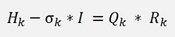
and
The value for the shifting is set to hnn for each loop.
Therefore the top of the function RunQR(..) is extended by
if (bShift)
phi
= m.a[order - 1, order - 1].real;
elsephi
=
0.0;
for
(i = 0; i < order; i++)m.a[i,
i].real = m.a[i, i].real - phi;
and RunRQ(..) gets the lines
for (i = 0; i < maxOrder; i++)
m.a[i,
i].real = m.a[i, i].real + phi;
at the end.
This modification improves the convergence behaviour of the QR transformation quite well.
When it comes to the calculation of conjugate complex eigenvalues, the explanations in the literature become very vague and fragmentary. And my approach finally became a bit different from what I read in this literature. Usually a double QR step with a complex shift is explained to compute complex eigenvalues. I don’t use that as it does not help for sure. If a matrix contains conjugate complex eigenvalues, the QR algorithm can behave in 3 different ways.
The 2x2 matrix mentioned is the matrix that consists of the last 2 rows and columns of the origin or reduced matrix like
and during QR transformation this matrix needs to be observed. The procedure is to check the element hn-1n (the second last element in the last row) if this element is 0 the computed eigenvalue will be real and can be calculated according to the description above. If it is not 0 there are 2 conjugate complex eigenvalues to be computed. In this case we have to check whether the values hn-1n-1, hn-1n, hnn-1 and hnn converge or not. If they converge we can go on with the QR transformation until they are accurate enough. Now we have to determine whether hn-1n-1, hn-1n, hnn-1 and hnn are conjugate complex eigenvalues or not. This can be found by comparing hn-1n, hnn-1 if their absolute value is equal and their sign is opposite, we have the eigenvalues. If not, we calculate the eigenvalues of the 2x2 matrix hn-1n-1, hn-1n, hnn-1 and hnn. If the values of hn-1n-1, hn-1n, hnn-1 and hnn do not converge, the story is not over. In this case we have to calculate the eigenvalues of the 2x2 matrix hn-1n-1, hn-1n, hnn-1 and hnn. And check if these values converge. If they do, we wait for them to be accurate enough and use them as our eigenvalues. All together it’s quite a complicate procedure. But it works. And that shows why a double QR step might not help in all the cases. It can improve the speed of convergence if the values converge. But if they do not converge, a double QR step does not help.
For this procedure I first implemented a function that calculates the eigenvalues of a 2x2 matrix:
public
void
CalcEigenvals22()
{
{
double
a, b, c;
a = 1.0;
b = -y[0, 0] - y[1, 1];
c = y[0, 0] * y[1, 1] - y[0, 1] * y[1, 0];
if ((b * b) >= (4.0 * a * c))
{
else
{
}a = 1.0;
b = -y[0, 0] - y[1, 1];
c = y[0, 0] * y[1, 1] - y[0, 1] * y[1, 0];
if ((b * b) >= (4.0 * a * c))
{
y[0,
0] =
(-b + Math.Sqrt((b
* b) - (4.0 * a * c))) /
2.0 / a;
y[1, 1] = (-b - Math.Sqrt((b * b) - (4.0 * a * c))) / 2.0 / a;
y[1, 0] = 0.0;
y[0, 1] = 0.0;
}y[1, 1] = (-b - Math.Sqrt((b * b) - (4.0 * a * c))) / 2.0 / a;
y[1, 0] = 0.0;
y[0, 1] = 0.0;
else
{
y[0,
0] =
-b / 2.0 / a;
y[1, 1] = y[0, 0];
y[0, 1] = Math.Sqrt((4.0 * a * c) - (b * b)) / 2.0 / a;
y[1, 0] = -y[0, 1];
}y[1, 1] = y[0, 0];
y[0, 1] = Math.Sqrt((4.0 * a * c) - (b * b)) / 2.0 / a;
y[1, 0] = -y[0, 1];
Then all the intelligence is in the function to check for convergence:
public
bool IsDeltoOk(int
order)
{
{
double
delta = 10.0;
double deltaEigen = 10.0;
bool result = false;
if (Math.Abs(m.a[order - 1, order - 2]) < 1E-20) // real eigenvalue
{
else
{
return result;
}double deltaEigen = 10.0;
bool result = false;
if (Math.Abs(m.a[order - 1, order - 2]) < 1E-20) // real eigenvalue
{
delta
=
m.a[order - 1, order - 1] - oldVal[0, 0];
oldVal[0, 0] = m.a[order - 1, order - 1];
result = Math.Abs(delta) < 1E-10;
}oldVal[0, 0] = m.a[order - 1, order - 1];
result = Math.Abs(delta) < 1E-10;
else
{
// convergence of the values themselves
y[0, 0] = m.a[order - 2, order - 2];
y[0, 1] = m.a[order - 2, order - 1];
y[1, 0] = m.a[order - 1, order - 2];
y[1, 1] = m.a[order - 1, order - 1];
delta = (y[0, 0] * y[0, 0] + y[0, 1] * y[0, 1]) -
oldVal[0, 1] = y[0, 1];
oldVal[1, 0] = y[1, 0];
oldVal[1, 1] = y[1, 1];
// convergence of the eigenvalues
CalcEigenvals22();
deltaEigen = (y[0, 0] * y[0, 0] + y[0, 1] * y[0, 1]) -
oldEigenVal[0, 1] = y[0, 1];
oldEigenVal[1, 0] = y[1, 0];
oldEigenVal[1, 1] = y[1, 1];
if (Math.Abs(delta) > Math.Abs(deltaEigen))
{
else
{
}y[0, 0] = m.a[order - 2, order - 2];
y[0, 1] = m.a[order - 2, order - 1];
y[1, 0] = m.a[order - 1, order - 2];
y[1, 1] = m.a[order - 1, order - 1];
delta = (y[0, 0] * y[0, 0] + y[0, 1] * y[0, 1]) -
(oldVal[0,
0] * oldVal[0, 0] + oldVal[0, 1] * oldVal[0, 1]) +
(y[1, 0] * y[1, 0] + y[1, 1] * y[1, 1]) -
(oldVal[1, 0] * oldVal[1, 0] + oldVal[1, 1] * oldVal[1, 1]);
oldVal[0,
0] = y[0, 0];(y[1, 0] * y[1, 0] + y[1, 1] * y[1, 1]) -
(oldVal[1, 0] * oldVal[1, 0] + oldVal[1, 1] * oldVal[1, 1]);
oldVal[0, 1] = y[0, 1];
oldVal[1, 0] = y[1, 0];
oldVal[1, 1] = y[1, 1];
// convergence of the eigenvalues
CalcEigenvals22();
deltaEigen = (y[0, 0] * y[0, 0] + y[0, 1] * y[0, 1]) -
(oldEigenVal[0,
0] * oldEigenVal[0, 0] + oldEigenVal[0, 1] *
oldEigenVal[0, 1]) +
(y[1, 0] * y[1, 0] + y[1, 1] * y[1, 1]) -
(oldEigenVal[1, 0] * oldEigenVal[1, 0] + oldEigenVal[1, 1] *
oldEigenVal[1, 1]);
oldEigenVal[0,
0] = y[0, 0];oldEigenVal[0, 1]) +
(y[1, 0] * y[1, 0] + y[1, 1] * y[1, 1]) -
(oldEigenVal[1, 0] * oldEigenVal[1, 0] + oldEigenVal[1, 1] *
oldEigenVal[1, 1]);
oldEigenVal[0, 1] = y[0, 1];
oldEigenVal[1, 0] = y[1, 0];
oldEigenVal[1, 1] = y[1, 1];
if (Math.Abs(delta) > Math.Abs(deltaEigen))
{
result = Math.Abs(deltaEigen)
< 1E-10;
}else
{
result = Math.Abs(delta)
< 1E-10;
}return result;
That looks like:
while
(actOrder > 1)
{
if (actOrder == 1)
{
{
delta
=
0;
RunQR(actOrder);
RunRQ(actOrder);
for (i = 0; i < actOrder; i++)
{
}RunQR(actOrder);
RunRQ(actOrder);
for (i = 0; i < actOrder; i++)
{
delta
=
delta + Math.Abs(oldVal[i]
- m.a[i,
i].real);
oldVal[i] = m.a[i, i].real;
}oldVal[i] = m.a[i, i].real;
if
(IsDeltoOk(actOrder))
{
}{
if
(actOrder > 1)
{
}{
if
(Math.Abs(m.a[actOrder
- 1, actOrder -
2].real) < 1E-20)
{
// real eigenvalue => record the real eigenvalue
actOrder -= 1;
}
else
{
}{
// real eigenvalue => record the real eigenvalue
actOrder -= 1;
}
else
{
if
(Math.Round(y[1,
0], 4) == -Math.Round(y[0,
1], 4))
{
else
{
actOrder -= 2;
}{
// complex eigenvalues in y
}else
{
// complex eigenvalues in the 2*2 matrix
}actOrder -= 2;
if (actOrder == 1)
{
// one last real eigenvalue in the first
diagonal element
}Computing the eigenvectors
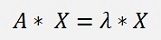
To compute the eigenvectors to the eigenvalues I use my own approach too In the literature they always explain the inverse vector iteration to compute eigenvectors. I tried that and it did not work. Then I spent a lot of time trying to find why it didn’t work and suddenly realized that I don’t need this inverse vector iteration. The formulation for the eigenvectors is:
or
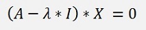
With λ as eigenvalue and X as an eigenvector.
This is a matrix equation that can be solved by a simple (little modified) Gaussian elimination algorithm (See Matrix Gauss)
For a 4*4 matrix this equation looks like:
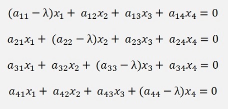
This matrix equation must be built and solved for each eigenvalue. It yields one eigenvector to the corresponding eigenvalue.
To solve this matrix equation we first have to build a right upper diagonal matrix and then we can solve the equations for the unknowns. Only, as all the equations are 0, we will not get absolute values but ratios between the values. Therefore we cannot just resolve the last equation for the last unknown x4 and have to set that to 1.0 to start. That looks like:
For a 4*4 matrix this equation looks like:
public void Solve()
{
int
k, l;
m.x[maxOrder - 1] = 1.0;
for (k = maxOrder - 2; k >= 0; k--)
{
}m.x[maxOrder - 1] = 1.0;
for (k = maxOrder - 2; k >= 0; k--)
{
for
(l = maxOrder - 1; l >= k; l--)
{
m.x[k] = m.y[k] / m.a[k, k];
}{
m.y[k]
=
m.y[k] - m.x[l] * m.a[k, l];
}m.x[k] = m.y[k] / m.a[k, k];
With m.y as the solution vector with staring value 0 for all elements and m.x as the eigenvector for one eigenvalue.
Now there is just one step left. As we can have complex eigenvalues, we can get complex eigenvalues as well. Therefore the Gaussian algorithm musst be implemented complex and it must be capable to yield complex results. Therefore I finally used a complex data type
public struct TComplex
{
public double real;
public double imag;
}
And use my static class MathComp this class and the data type are implemented in the module TComplex.cs. The complex Gaussian algorithm is implemented in TGauss.cs and the complex Matrix I use is defined in TMatrix.cs.
In the literature they also mention the Frobenius matrix to be used for the decomposition. I implemented this algorithm to and was very convinced by it in the beginning. It is quite a lean and elegant algorithm. But it’s convergence behaviour is not too reliable. There are situations it converges very well. But quite often it does not. Therefore I abandoned this approach finally