


An eigenvector is a vector X that is multiplied by the matrix A equal to a fixed value λ (the eigenvalue of A to this eigenvector) multiplied by the same vector X
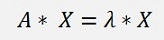
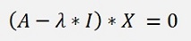
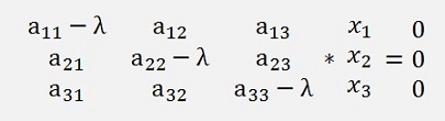
This is a matrix equation that can be written as
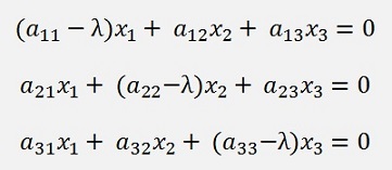
As example for a 3x3 matrix with x1…x3 the eigenvector and λ as the eigenvalue to the eigenvector.
To a N*N matrix there exist N eigenvalues and N eigenvectors.
To compute the eigenvalues of small matrixes the approach using the characteristic polynomial is a good Joyce. I first used this approach on a 2*2 matrix in my QR algorithm. So I start whit this here:
The equation for the eigenvalues and eigenvectors for a 2*2 matrix looks like:
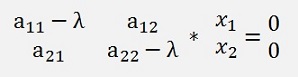
The condition that this matrix equation has a solution is that the determinant of A is 0 and with this condition we can work. The determinant of A is
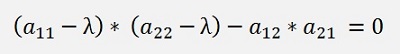
this equation expanded

This is the characteristic polynomial to the matrix A
and it can be solved as a quadratic equation
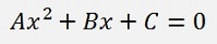
(See Quadratic equation)
And the solution for this equation is
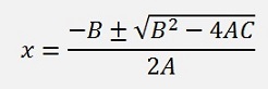
With the possibility that B2 – 4AC can be < 0 and the solution is complex this can be put into a function:
public void CalcEigenvals()
{
double
a, b, c;
a = 1.0;
b = -m[0, 0] - m[1, 1];
c = m[0, 0] * m[1, 1] - m[0,1] * m[1, 0];
if ((b * b) >= (4.0 * a * c))
{
else
{
}a = 1.0;
b = -m[0, 0] - m[1, 1];
c = m[0, 0] * m[1, 1] - m[0,1] * m[1, 0];
if ((b * b) >= (4.0 * a * c))
{
y[0,
0] =
(-b + Math.Sqrt((b
* b) - (4.0 * a * c))) /
2.0 / a;
y[0, 1] = (-b - Math.Sqrt((b * b) - (4.0 * a * c))) / 2.0 / a;
}y[0, 1] = (-b - Math.Sqrt((b * b) - (4.0 * a * c))) / 2.0 / a;
else
{
y[0,
0] =
-b / 2 / a;
y[0, 1] = y.a[0, 0];
y[1, 0] = Math.Sqrt((4.0 * a * c) - (b * b)) / 2.0 / a;
y[1, 1] = -y.a[1, 0];
}y[0, 1] = y.a[0, 0];
y[1, 0] = Math.Sqrt((4.0 * a * c) - (b * b)) / 2.0 / a;
y[1, 1] = -y.a[1, 0];
And the solution for this equation isThis function gets the 2*2 matrix in m, computes the eigenvalues of it and returns them in the 2*2 matrix y. If the eigenvalues are real, they will be in y[0,0] and y[0,1], if they are complex, the imaginary part to y[0,0] will be in y[1,0] and the imaginary part to y[0,1] will be in y[1,1]. That was quite easy
But if the matrix becomes bigger, things become much more complicate with this approach. I did the same for a 3*3 matrix like
The formulation for the determinant for this matrix is
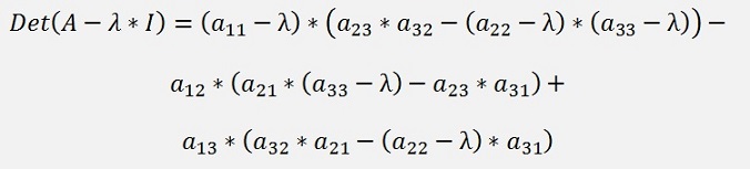
And this is the characteristic polynomial for A again. To expand this and bring it to the form
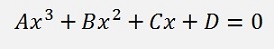
is a hell of a calculation
It ends with
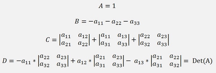
Now we can use Cardano’s method to solve a cubic equation (See Cardano)
In my sample project I just initialise the values of a, b, c and d and call the function I already implemented in the sample project of the Cardano Algorithm:
a1 = 1.0;
b = -(m[0, 0] + m[1, 1] + m[2, 2]);
c = m[0, 0] * m[1, 1] - m[0, 1] * m[1, 0] + m[0, 0] * m[2, 2] –
m[0, 2] * m[2, 0] + m[1, 1] * m[2, 2] - m[1, 2] * m[2, 1];
d = -m[0, 0] * (m[1, 1] * m[2, 2] - m[1, 2] * m[2, 1]) +
m[0, 1] * (m[1, 0] * m[2, 2] - m[1, 2] * m[2, 0]) –
m[0, 2] * (m[1, 0] * m[2, 1] - m[1, 1] * m[2, 0]);
if ((a1 != 0) && (b != 0) && (c != 0) && (d != 0))
{
Calc_Cardano();
}O.k. the approach using the characteristic polynomial is quite neat for small matrixes up to 3x3. If the matrix is bigger the topic eigenvalue immediately becomes much more complicate and cannot be calculated like this anymore. For bigger matrixes iterative approaches applying similarity transformations are used. The case of a symmetric matrix which has only real eigenvalues is the easiest situation then and can be solved by the use of a Jacoby transformation. The most complicate case is a random matrix that contains real and complex eigenvalues and has to be solved by a QR transformation which is the most complex but also most stabile algorithm for such a case. There is also the LU decomposition that can be used to compute eigenvalues of a random matrix. But it does not work in all cases if it is to compute the eigenvalues of a random matrix. But it’s a very interesting approach to compute the roots of a polynomial and there it works quite well
Basically a similarity transformation transforms a matrix into an upper triangle matrix by multiplying it by transposed rotation matrixes in a first step and transforms it back by multiplying it by the rotation matrixes. This is repeated in a loop and at the end of each loop the elements in the main diagonal of the transformed matrix get a bit closer to the eigenvalues of the matrix and the elements below become 0. At the end the matrix remains as an upper triangle matrix if there are only real eigenvalues and the eigenvalues are the elements in the main diagonal. If there are complex eigenvalues the matrix becomes a quasi upper triangle matrix and not all the elements below the main diagonal will be 0 as shown here
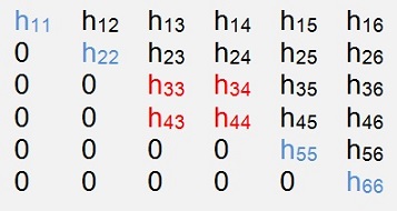
The blue elements are real eigenvalues and the red 2*2 matrix holds a pair of conjugate complex eigenvalues. But more to this in
Eigenvalues of a symmetric matrix by Jacobi
QR decomposition to compute real and complex Eigenvalues and eigenvectors of a matrix
(see also Vector iteration)