

The vector iteration is the simplest way to compute one single, real Eigenvalue. The outcome of the vector iteration is an eigenvector to which the eigenvalue can be computed. Usually it finds the eigenvector with the eigenvalue that has the biggest absolute value (but that’s not for sure
 )
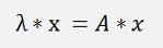
)Starting from the basic formulation for eigenvalues and their eigenvectors (see Eigenvalues basics)
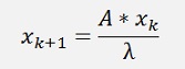
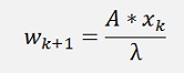
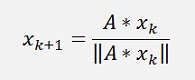
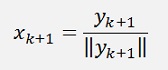
If the eigenvalue is taken to the right side the formulation for xk+1 is:
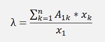
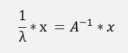
if we just use one row of A we get for λ
The formulation for the iteration means there is a multiplication of the matrix A with the vector xk. The result of this is another vector xk+1 and this one is divided by λ and then it is used for the next iteration. And λ is calculated as mentioned above and if it does not change anymore, the vector iteration has converged and we have got the eigenvector in x and the eigenvalue in λ.
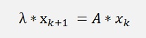
The iteration starts with a random eigenvector and looks like:
public void RunVector(int maxOrder)
{
int i, k, count = 0;
double[] x2 = new double[maxOrder];
double[] y = new double[maxOrder];
double delta = 10;
double oldZ = 1E30;
while ((delta > 1.0E-50) && (count < 150))
{
}double[] x2 = new double[maxOrder];
double[] y = new double[maxOrder];
double delta = 10;
double oldZ = 1E30;
while ((delta > 1.0E-50) && (count < 150))
{
count++;
// multiplication A * xn
x2 = MultMatrixRight(a, x1, maxOrder);
for (i = 0; i < maxOrder; i++)
{
// calculate the eigenvalue
eigenval = 0;
for (i = 0; i < maxOrder; i++)
{
eigenval = eigenval / maxOrder;
// set xn+1 for the next iteration
for (i = 0; i < maxOrder; i++)
{
// check the delta between the last iteration and the current
delta = Math.Abs(oldZ - eigenval);
oldZ = eigenval;
}// multiplication A * xn
x2 = MultMatrixRight(a, x1, maxOrder);
for (i = 0; i < maxOrder; i++)
{
y[i] = 0;
for (k = 0; k < maxOrder; k++)
{
}for (k = 0; k < maxOrder; k++)
{
y[i] = y[i] + a[k, i] * x1[k];
}// calculate the eigenvalue
eigenval = 0;
for (i = 0; i < maxOrder; i++)
{
eigenval = eigenval + y[i] / x1[i];
}eigenval = eigenval / maxOrder;
// set xn+1 for the next iteration
for (i = 0; i < maxOrder; i++)
{
x1[i] = x2[i] /
eigenval;
}// check the delta between the last iteration and the current
delta = Math.Abs(oldZ - eigenval);
oldZ = eigenval;
This function gets an initial eigenvector in the array x1 and the array to compute the eigenvalues from in the array a. It uses the function
public double[] MultMatrixRight(double[,] a, double[] z, int size)
{
int i, k;
double[] al = new double[size];
for (i = 0; i < size; i++)
{
return al;
}double[] al = new double[size];
for (i = 0; i < size; i++)
{
al[i] = 0.0;
for (k = 0; k < size; k++)
{
}for (k = 0; k < size; k++)
{
al[i] = al[i] +
(a[i, k] * z[k]);
}return al;
With a sample matrix of
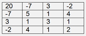
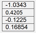
I get the Eigenvalue 23.527
And the eigenvector
To avoid an overflow or underflow of the eigenvector it is principally a good idea to normalize the eigenvector in each iteration by dividing it by its length. That would be:
and
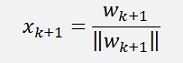
Whereas ||wk+1|| is the length of the vector wk+1 But instead of dividing by λ and additionally by ||wk+1|| we can say it’s as good just to divide by the length of the eigenvector. That’s enough and the algorithm converges even better.
Or with the auxiliary variable wk+1:
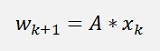
and
And that’s what the current literature describes as the vector iteration.
According to what’s written in the literature the division by ||wk+1|| is a normalization of wk+1 to avoid an overflow or underflow during iteration.
I say this ||wk+1|| contains λ (even if that’s not too obvious) and the algorithm would not work without this division. ||wk+1|| is used in place of λ * ||wk+1|| to simplify the algorithm and to improve its ability to converge.
Basically the above implementation is rather complicate and does not make too much sense. But I think it is quite interesting for the understanding of the vector iteration as this is straight according to the formulation and the descriptions that can be found in the net are not too clear about this derivation.
Now the real implementation uses just ||A * xk|| for the normalisation of the eigenvector. That’s much more elegant
.And that gives the following procedure:
public void RunVector(int maxOrder)
{
int i, k, count = 0;
double[] x2 = new double[maxOrder];
double[] y = new double[maxOrder];
double delta = 10;
double oldZ = 1E30;
double lenW = 0;
while ((delta > 1.0E-50) && (count < 50))
{
// calculate the eigenvalue
for (i = 0; i < maxOrder; i++)
{
eigenval = 0;
for (i = 0; i < maxOrder; i++)
{
eigenval = eigenval / maxOrder;
}double[] x2 = new double[maxOrder];
double[] y = new double[maxOrder];
double delta = 10;
double oldZ = 1E30;
double lenW = 0;
while ((delta > 1.0E-50) && (count < 50))
{
count++;
x2 = MultMatrixRight(a, x1, maxOrder);
lenW = 0.0;
// calculate the length for normalisation
for (i = 0; i < maxOrder; i++)
{
lenW = Math.Sqrt(lenW);
// normalisation of the eigenvector
for (i = 0; i < maxOrder; i++)
{
delta = Math.Abs(oldZ - lenW);
oldZ = lenW;
}x2 = MultMatrixRight(a, x1, maxOrder);
lenW = 0.0;
// calculate the length for normalisation
for (i = 0; i < maxOrder; i++)
{
lenW = lenW + x2[i] * x2[i];
}lenW = Math.Sqrt(lenW);
// normalisation of the eigenvector
for (i = 0; i < maxOrder; i++)
{
x1[i] = x2[i] / lenW;
}delta = Math.Abs(oldZ - lenW);
oldZ = lenW;
// calculate the eigenvalue
for (i = 0; i < maxOrder; i++)
{
y[i] = 0;
for (k = 0; k < maxOrder; k++)
{
}for (k = 0; k < maxOrder; k++)
{
y[i] = y[i] + a[k, i] * x1[k];
}eigenval = 0;
for (i = 0; i < maxOrder; i++)
{
eigenval = eigenval + y[i] / x1[i];
}eigenval = eigenval / maxOrder;
To check if the calculation is accurate enough I use the length of x2 here. If that does not change anymore the computation is finished.
With a sample matrix of
I get the Eigenvalue 23.527
And the eigenvector
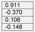
I use a symmetric matrix to make sure I get a real eigenvalue as this implementation of the Vector Iteration can only find real eigenvalues.
With these sample values here it finds the eigenvalue with the biggest absolute value. But if the matrix is not symmetric that can be different
.
Inverse Vector iteration
And with this it finds the biggest inverse value of an eigenvalue and that would be the smallest if it is not inverse. I tried that and it did not work
The above sample has the eigenvalues
The first two values have absolute values very close to each other. That seems to be too close for the vector iteration and so the algorithm did not work with the inverse matrix. I think that’s the weakness of the vector iteration. It does not converge too well if the absolute values of the eigenvalues are too close to each other.
(but anyhow for the inverse of a matrix see Inverse matrix)
The behaviour of the inverse vector iteration can be improved if a so called shift value is used. If the eigenvalues of the matrix A are “shifted” by a value close to an eigenvalue, it converges quite well. To shift means to subtract a shift-value µ from all main diagonal elements of the matrix A. In a formula this is written as µ*I (I is the identity matrix) subtracted from A.
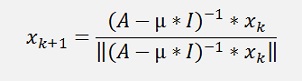
We can build the inverse matrix of A - µ*I and multiply this by xk.
But the second approach is more elegant. It says
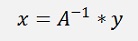
Is the same as solving the matrix equation
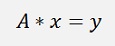
For x.
And that can be done by a Gaussian elimination algorithm.
So, with x set to yk+1 and y set to xk, the algorithm becomes:
To solve the matrix equation
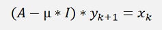
Normalize yk+1 and set this as xk+1
The eigenvalue is calculated according to (same as above)
And repeat the iteration as long as the eigenvalue changes.
I implemented this into this C# function:
private void RunVector(TMatrix m)
{
int i, k;
double len = 0.0;
double[] y = new double[MaxOrder];
gauss = new TGauss(MaxOrder, m);
for (i = 0; i < MaxOrder; i++)
{
gauss.Eliminate();
gauss.Solve();
// calculate the length of x
len = 0;
for (i = 0; i < MaxOrder; i++)
{
len = Math.Sqrt(len);
// narmalize the eigenvector and set y for the next loop
for (i = 0; i < MaxOrder; i++)
{
// calculate the eigenvalue
for (i = 0; i < MaxOrder; i++)
{
eigenvalue = 0;
for (i = 0; i < MaxOrder; i++)
{
eigenvalue = eigenvalue / MaxOrder;
}double len = 0.0;
double[] y = new double[MaxOrder];
gauss = new TGauss(MaxOrder, m);
for (i = 0; i < MaxOrder; i++)
{
for (k = 0; k < MaxOrder; k++)
{
m.a[i, i] = m.a[i, i] - shift;
m.x[i] = 0;
}{
m.a[k, i] = ori.a[k, i];
}m.a[i, i] = m.a[i, i] - shift;
m.x[i] = 0;
gauss.Eliminate();
gauss.Solve();
// calculate the length of x
len = 0;
for (i = 0; i < MaxOrder; i++)
{
len = len + m.x[i] * m.x[i];
}len = Math.Sqrt(len);
// narmalize the eigenvector and set y for the next loop
for (i = 0; i < MaxOrder; i++)
{
eigenVect[i] = m.x[i] / len; // eigenvector
to u
m.y[i] = eigenVect[i]; // set y for the next iteration
}m.y[i] = eigenVect[i]; // set y for the next iteration
// calculate the eigenvalue
for (i = 0; i < MaxOrder; i++)
{
y[i] = 0;
for (k = 0; k < MaxOrder; k++)
{
}for (k = 0; k < MaxOrder; k++)
{
y[i] = y[i] + ori.a[k, i] * eigenVect[k];
}eigenvalue = 0;
for (i = 0; i < MaxOrder; i++)
{
eigenvalue = eigenvalue + y[i] / eigenVect[i];
}eigenvalue = eigenvalue / MaxOrder;
Here I use y of my matrix class instead of x1 and solve the matrix equation A*x = y by a Gaussian elimination algorithm. The matrix class contains A, X and Y as arrays.
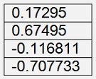
With this implementation and the same sample as above
and a starting value µ = -2
I get the Eigenvalue -1.16095
and the eigenvector
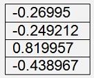
and with a starting value µ = 2
I get the Eigenvalue 1.17305
with the eigenvector
It is basically possible to find every eigenvalue as long as the starting value of µ is close enough to it. But this is in my opinion the big disadvantage of this algorithm: You need to know the approximate value of the eigenvalue you are looking for. Therefore I think it might be smarter to use a QR decomposition algorithm and compute all eigenvalues at once
(see Eigenvalues QR
decomposition and Eigenvalues of a symmetric matrix by Jacobi)