Mosi's Math

Differential equation by Runge Kutta and Heun

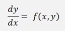
Carl Runge and Wilhelm Kutta developed a family of methods to solve an ordinary differential equation of the form:

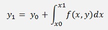
The idea is to calculate y for a random x and therefore the basic formulation for an iterative approximation of y by Runge and Kutta is

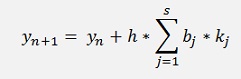
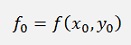
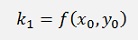
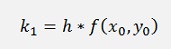
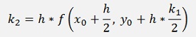
With h = step size and

...

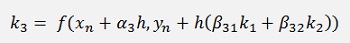
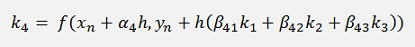
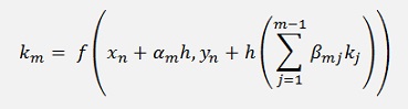
That looks quite complicate but fortunately not all formulations use all numbers of k.

Method of Heun

The method of Karl Heun is similar to the second order Runge Kutta algorithm. It integrates both sides of the above formula to

And as

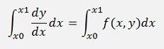
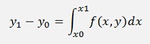
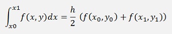
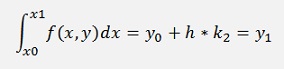
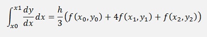
Now the definite integral is solved by the trapezoidal rule

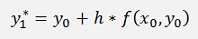
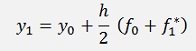
and as the linearization of Euler says

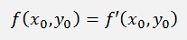
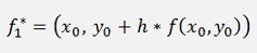
and due to that we can approximate y₁ to y₁*

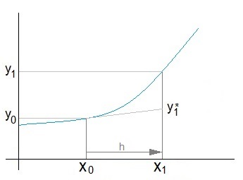
That looks quite inaccurate but with a small step size it’s not too bad :-)

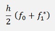
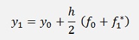
This inserted in the above formula gives:

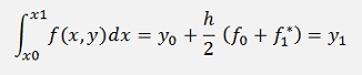
With

That’s the formulation of the Heun algorithm.

Second order Runge Kutta

From a different view we can say

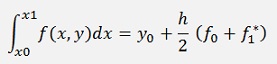
is an approximation with the trapezoidal integration rule that uses the trapezoidal

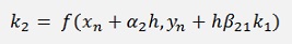
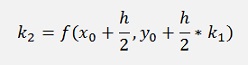
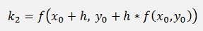
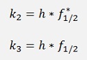
Instead of this we can as well use the function value on the half way from x₀ to x₁ multiplied by h like

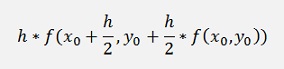
with this we get the formulation of the second order Runge Kutta algorithm:

and

Implemented in a small loop the Heun algorithm looks like:

int i;
double h = 1.0 / (double)(datapoints-1);
double k1, k2;
xp[0] = 0;
yp[0] = 1; // initial value for y[0]
for (i = 1; i < datapoints; i++)
{
     xp[i] = i * h;
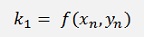
     k1 = f_xy(xp[i - 1], yp[i - 1]);
     yp[i] = yp[i - 1] + h/2 * (k1 + f_xy(xp[i], yp[i - 1] + h * k1));
}

For the implementation of the second order Runge Kutta algorithm the last line in the loop must be replaced by the 2 lines

k2 = f_xy(xp[i - 1] + h / 2, yp[i - 1] + h / 2 * k1);

yp[i] = yp[i - 1] + h * k2;

In my sample project I implemented the equation

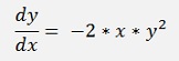
With the initial value y(0) = 1

Which has the exact solution

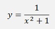
And so

double f_xy(double x, double y)
{
return -2 * x * y * y;
}

With this the exact solution for x = 1 is y = 0.5 The algorithm by Heun returns 0.50000982 and the Runge Kutta approach returns 0.499998 with 100 supporting points.

Fourth order Runge Kutta

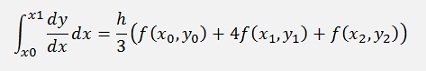
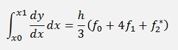
Similar to the Heun algorithm, the 4. Order Runge Kutta algorithm integrates the main formula

But the definite integral is not solved by the trapezoidal method but the Simpson integral (see Simpson integration for a detailed description)

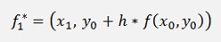
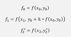
For this approach y₁ and y₂ must be computed somehow. Therefore y₁ is approximated according to Heun as y₁* = y₀ + h*f(x₀). This will be used later on.

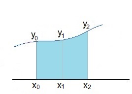
With 3 supporting points we can set up a 3. order polynomial to approximate the function f(x) within the interval x₀ to x₂. That leads to the following 4 equations:

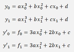
whereas

Now the basic approach would be to solve this matrix equation. But that would end in a hell of a calculation.

A more suitable way to proceed is to do a parameter comparison:

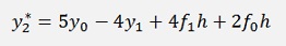
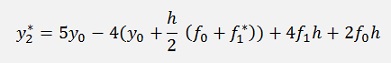
At the end we need the solution for the approximation of y₂:

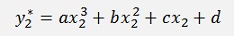
which can be written as:

or expanded:

From this equation a, b, c and d should vanish as they are unknown.

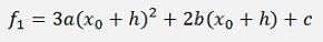
Therefore I first try to get rid of the h³ term in the a part.

If we have a look on a term

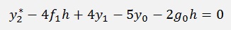
If this is subtracted from the equation for y₂*

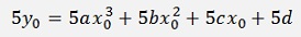
Some parts already vanished. But there is still 5x₀³ in the a part. That’s 4 too much. So I subtract 5y₀

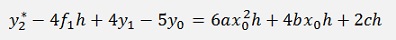
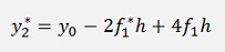
Now it’s easy to see that there is only the subtraction of 2g₀h that remains:

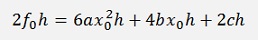
and with this

and according to Heun

If this is inserted in the above formula we get

Or simplified

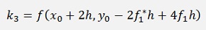
with

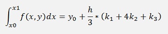
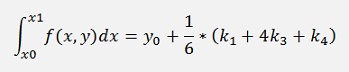
Now everything can be put together in the Simpson formula

With the approximation for y₂ we have

with

Or in the Runge Kutta form

with

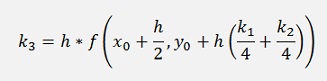
Now there is only one thing the remains: With this formulation h = (x₁ – x₀)/2. But we need h = (x₁ – x₀). That means we have to divide every h from above by 2 and get

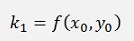
With

and with

and as

In a small c# sequence that looks like:

double h = 1.0 / (double)(datapoints - 1);
double k1, k2, k3, k4;

xp[0] = 0;
yp[0] = 1; // initial value for y[0]
for (i = 1; i < datapoints; i++)
{
     xp[i] = i * h;
     k1 = f_xy(xp[i - 1], yp[i - 1]);
     k2 = f_xy(xp[i - 1] + h / 2, yp[i - 1] + h * k1 / 2);
     k3 = f_xy(xp[i - 1] + h / 2, yp[i - 1] + h * (k1 + k2) / 4);
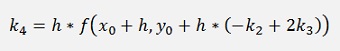
     k4 = f_xy(xp[i - 1] + h, yp[i - 1] + h * (-k2 + 2 * k3));
     yp[i] = yp[i - 1] + h / 6 * (k1 + 4 * k3 + k4);
}

That looks quite similar to the second order Runge Kutta algorithm. But a comparision of the two’s shows the difference:

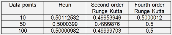
With its polynomial approximation the fourth order Runge Kutta algorithm is already quite accurate with just a few data points or a rather big step width between two data points. That makes it quite attractive as it is not too much more complicate to be implemented than the other two’s :-)

C# Demo Project to Runge Kutta algorithm

RungeKutta4.zip