

The Runge Kutta algorithms are very interesting methods to solve an ordinary differential equation of the form:
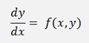
(see Differential equation by Runge Kutta and Heun for a detailed description)
But the approximation by the Runge Kutta algorithm can become inaccurate if the function to approximate is irregular bended.
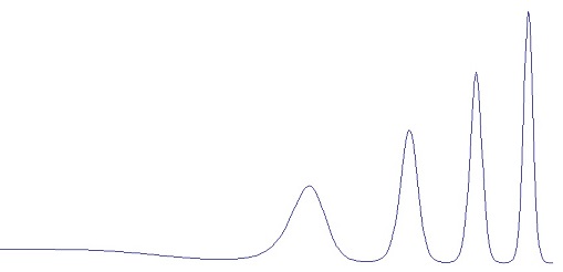
To approximate a curve like this the step width of the algorithm would have to be set to a relatively small size and due to that the calculation becomes time consuming.
To avoid this the Runge Kutta algorithm can be implemented with adaptive step size. With such an approach the algorithm can proceed with a bigger step size in flatter areas of the curve and with smaller step size in bended areas. That safes a lot of calculation time without losing too much accuracy.
To determine whether the step size can be increased or has to be decreased a good approach is to compare a higher order Runge Kutta algorithm to a lower order Runge Kutta algorithm. If the difference between these two’s is too big, the step size should be reduced. If the difference is small, the step size can be increased.
To reduce the calculation effort it is whise to use to Runge Kutta algorithms that have as many k-parameters the same as possible.
In the literature it is usually said that a lower order Runge Kutta should be compared to a higher order one. I think it is as well possible to do it inverse and use the higher order for the approximation and the lower order for comparison.
As I already implemented the second order and the fourth order Runge Kutta algorithm, I use these two’s for the implementation of an adaptive one. I do the approximation by the fourth order Runge Kutta and use the second order one for comparison.
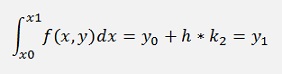
The second order Runge Kutta algorithm has the formulation
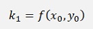
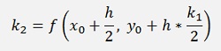
and
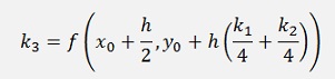
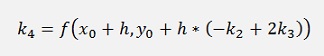
The fourth order Runge Kutta has
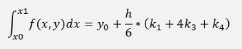
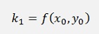
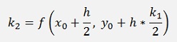
with
So the difference between both is
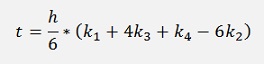
Now, the correct threshold to adapt the step size must be determined according to the function that shall be approximated.
In my sample project I use the function
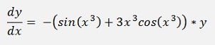
With initial values x(0) = 0 and y(0) = 1.
The approximation of this equation creates the above graph. For this function I can divide the step size by 2 if t is bigger than 0.1 and I multiply it by 2 if t is smaller than 1E-10. With this setting I can start with a step size of 0.5. The algorithm reduces this step size to 0.0078125 during approximation. At x = 3 the exact value for y = 0. With the adaptive step size I get y = 0.05640768 with 109 steps. The fourth Order Runge Kutta algorithm with fixed step size needs 400 steps to get 0.05695618. That’s more than 3 times as much. With 109 steps it gets 0.22353683 which is quite a bit less accurate.
The adaptive version of the fourth order Runge Kutta algorithm looks a little more complex than the one using a fixed step size:
private void CalcRungeKuttaVar()
{
int i=1;
double h = hMax;
double hp = 3.0 / (double)(datapoints - 1);
double k1, k2, k3, k4;
double t = 0;
int count = 0;
bool updateValues = true;
for(i = 0; i < datapoints; i++)
{
xp[i] = 0;
yp[i] = 0;
}
i = 1;
// initial values
x = 0;
y = 1;
xp[0] = x;
yp[0] = y;
while (x < 3)
{
k1 = f_xy(x, y);
k2 = f_xy(x + h / 2, y + h / 2 * k1);
k3 = f_xy(x + h / 2, y + h * (k1 + k2) / 4);
k4 = f_xy(x + h, y + h * (-k2 + 2 * k3));
t = h / 6 * (k1 + 4 * k3 + k4 - 6 * k2);
updateValues = true;
if (Math.Abs(t) > 5E-2)
{
if (h > hMin)
{
h = h / 2;
updateValues = false;
}
}
else
{
if (Math.Abs(t) < 1E-10)
{
if (h < hMax)
{
h = h * 2;
updateValues = false;
}
}
}
if(updateValues)
{
count++;
y = y + h / 6 * (k1 + 4 * k3 + k4);
x += h;
if ((x - (i * hp) > 0) && (i < datapoints))
{
xp[i] = x;
yp[i] = y;
i++;
}
}
}
}
And the fixed version
private void CalcRungeKutta4()
{
int i;
double h = 3.0 / (double)(datapoints - 1);
double k1, k2, k3, k4;
// initial values
x = 0;
y = 1;
for (i = 1; i < datapoints; i++)
{
k1 = f_xy(x, y);
k2 = f_xy(x + h / 2, y + h * k1 / 2);
k3 = f_xy(x + h / 2, y + h * (k1 + k2) / 4);
k4 = f_xy(x + h, y + h * (-k2 + 2 * k3));
y = y + h / 6 * (k1 + 4 * k3 + k4);
x += h;
xp[i] = x;
yp[i] = y;
}
}
{
int i;
double h = 3.0 / (double)(datapoints - 1);
double k1, k2, k3, k4;
// initial values
x = 0;
y = 1;
for (i = 1; i < datapoints; i++)
{
k1 = f_xy(x, y);
k2 = f_xy(x + h / 2, y + h * k1 / 2);
k3 = f_xy(x + h / 2, y + h * (k1 + k2) / 4);
k4 = f_xy(x + h, y + h * (-k2 + 2 * k3));
y = y + h / 6 * (k1 + 4 * k3 + k4);
x += h;
xp[i] = x;
yp[i] = y;
}
}
with
double f_xy(double x, double y)
{
return -(Math.Sin(x*x*x)+3*x*x*x*Math.Cos(x*x*x))*y;
}