

The radial basis functions network can be used to approximate a multidimensional function of a set of input vectors X and their output y. It looks a bit like a neural net. But it isn’t and it does not work as well as a neural net does.
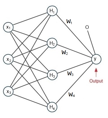
A simple radial basis functions network
Usually the radial basis functions network has 3 layers: An input layer, a hidden layer and an output layer. The hidden layer normally has more knots than the input layer and quite often the output layer has only one knot and builds the function.

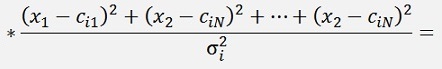
With
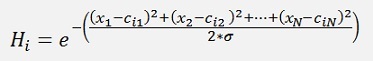
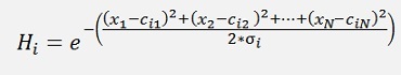
Where Ci is called prototype or center point of the ith knot and
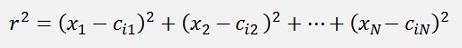
and
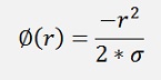
Is the radial basis function.
There are other radial basis functions used in other applications. But here I use just this one. It is called “Gaussian radial basis function”. The factor σ in some articles is said to be the standard deviation of the vectors X around the centers C. I say it’s not really like that

To find an approximating function to the input data X there are several approaches. It think the simplest and most efficient one is to separate the data into clusters and use the centre points of these clusters as C points (C has always the same amount of dimensions as X). With this the hidden layer gets as many knots as clusters have been built.
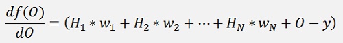
Whit these clusters the net must be trained to find a setting of the weights W, the offset O and σ. This is done with the Gradient descend (see Gradient descend for a detailed description) method and cost-function
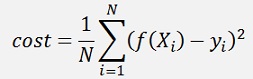
With N as the number of data samples and Xi and yi one data sample.
For the Gradient descend the differentiation
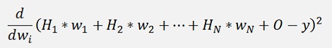
must be built.
With the chain rule (see Differential calculus) the differentiation with respect to wi is not too complicate:
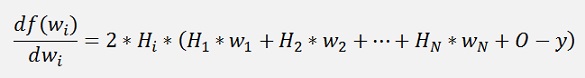
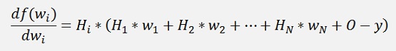
Whereas the multiplication by 2 can be neglected:
For the offset it’s even simpler:
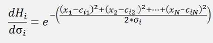
and finally there is σ. For σ the differentiation is a bit more complicate:
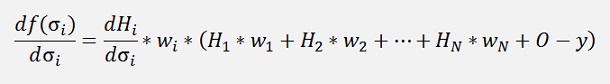
and with
we get
This inserted in the above formulation:
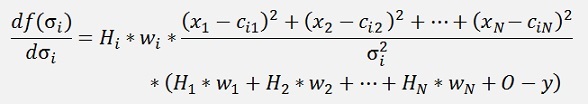
Quite a formula
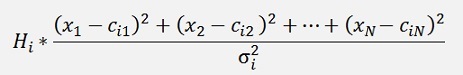
For the implementation of this algorithm first we need to cluster the input data (see Clustering data by a K-means algorithm) . With the center points of the computed clusters Hi can be computed like:
public void CalculateH(double[] x, Collection<Cluster> cluster)
{
int j, k;
for (j = 0; j < H.Length; j++)
{
radialF[j] = 0;
for (k = 0; k < x.Length; k++)
{
radialF[j] += (x[k] - cluster[j].centerPoint[k]) * (x[k] - cluster[j].centerPoint[k]);
}
H[j] = Math.Exp(-radialF[j] / sigma);
}
}
The variable radialF is the Φ from above. I changed the name to avoid confusion with the number Φ.
With Hi the Gradient can be computed:
public double CalculateGradient(double[] x, double y)
{
int i;
double tempSum = 0;
for (i = 0; i < featuresIn; i++)
tempSum += H[i] * w[i];
for (i = 0; i < featuresIn; i++)
{
gradient[i] += H[i] * (tempSum + offs - y);
deltaSigma += H[i] * (tempSum + offs - y) *w[i] * radialF[i] / sigma / sigma;
}
deltaOffs += (tempSum + offs - y);
return (tempSum + offs - y) * (tempSum + offs - y);
}
This function computes the Gradient of W and the change for σ and the offset and it returns the part of the cost that is generated by the sample (X, y).
In one iteration the function CalculateH and CalculateGradient must be called for all samples. That gives the changes for W, σ and the offset to be subtracted in the next step:
public void UpdateValues(int samples, double learning_rate)
{
int i;
for (i = 0; i < featuresIn; i++)
{
w[i] -= gradient[i] / samples * learning_rate;
}
sigma -= deltaSigma / samples * 10;
offs -= deltaOffs / samples * learning_rate;
}
Approximation using radial basis functions
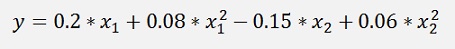
In the sample project I use a data set I created for this algorithm. It consists of data points computed with the 2 dimensional function:
To get a useful clustering there are 7 center points with some data points around them.
The 7 center points are
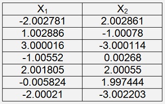
And they are stored in the file Centerpoint.csv The distribution looks like:
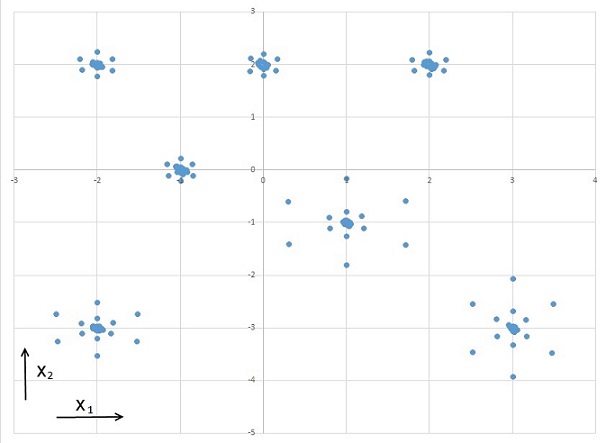
They should represent a set of measuring points with some inaccuracy. There are 144 data points with a random noise within ±0.01. That makes y-values between -0.16759 and 2.899164 and these y-values are the values to be approximated.This is done by the sequence:
public class TData
{
public Collection<double[]> values = new Collection<double[]>();
public int dataLength = 0;
public void readData(string FileName)
{
foreach (var str in File.ReadLines(FileName, Encoding.Default))
{
int i;
string[] strLine = str.Split(',');
double[] line = new double[strLine.Length];
for (i = 0; i < strLine.Length; i++)
line[i] = Convert.ToDouble(strLine[i]);
dataLength = line.Length;
values.Add(line);
}
}
}
Whit this sequence carried out 1000 000 times the algorithm yields:
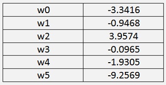
Offset = 18.0268
σ = 122.0778
and
cost = 0.00034957
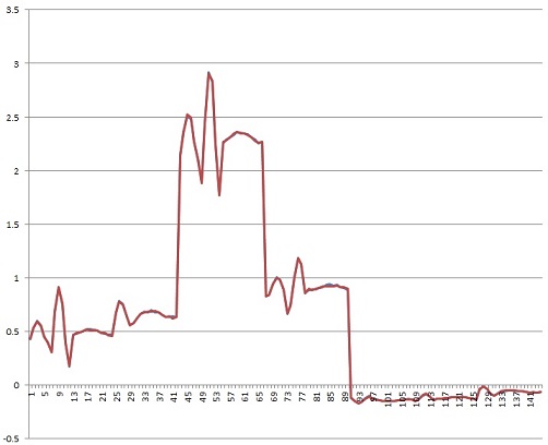
This cost value looks quite good. But if we compare the approximated values (the blue curve) to the reference values (the red curve), obviously not all values are approximated that well.
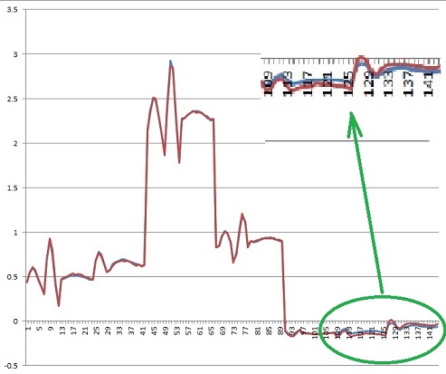
Beginning at the data point 109 all the rest of the data points are relatively bad approximated. There is quite some difference between the 2 curves. That’s not too useful.
Using the Gradient descend algorithm (see Gradient descend) to approximate the same data, the result is much better.
If the algorithm is implemented with the target function

With this target function and 2110 iterations with the learning_rate = 0.001 the Gradient descend algorithm got the approximation

With a cost = 1.671E-05That looks much better
The graphic shows:
It approximates the origin shape (blue and invisible below the red shape) without noise very nice. As the very small cost already suggests
Another interesting approach could be the Method of the least squares multi-dimensional.