

In machine learning the Gradient Descend or Backpropagation algorithm are widely used approaches. Both try to approximate a function onto a set of given data samples. The Support Vector Machine is a different approach. It tries to classify data. For this classification it tries to lay plane between two groups of the data. Imagen we have a set of data points (x1, x2, y) in 2 dimensional space that have a value y = 1 (red) and y = -1 (blue). These points can be separated by a line (the black line). Additionally there should be some gap to make sure other data points will be classified correct later on. This gap is marked by the two grey lines. In multi-dimensional spaces there 3 lines are hyperplanes.
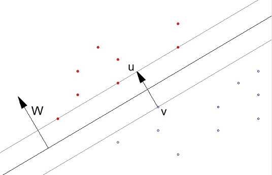
For the moment we assume that the data is separable by a straight line. The case that it can’t, will be treated further down.
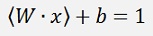
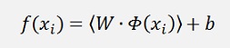
What the algorithm does is, it determines a vector the W which is perpendicular to the separating line (or hyperplane). Now as the dot product of 2 vectors is their lengths multiplied and the result of this multiplication multiplied by the cosine of the angle between these 2 vectors, in the case the separating line would lead through the zero-point, the dot product of W and a random data point would be >0 if the data point lays above the separating line and it would be <0 if the data point lays below the this line. But as the separating line most probably does not run through the zero-point, a constant factor b is add and we get the formulation
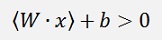
For data points laying above the separating (with y = 1) line and
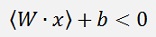
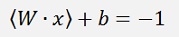
For data points below the separating line (with y = -1).
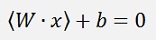
For data points laying on the separating line
That’s one part of the task. The second part is to determine the gap that should be between the separated classes (the grey lines). This gap shall be as big as possible to have a maximised possibility that later data will be classified correct.
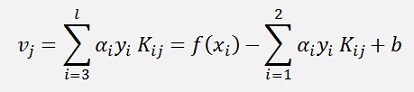
This gap is basically the vector u-v and this vector should be as long as possible. In 2 dimensional spaces that can be reached be placing the line as it is in the graphic above. That would be quite easy and there is an algorithm named “nearest point algorithm” that does this. That might work fine in 3 dimensional spaces to. But try to imagen how that should be done in case of more dimensional spaces. I’m not too convinced of this approach

In a numerical algorithm W is basically determined that
for points that lay on the upper grey line and
for points laying on the lower grey line.
Here, for the nearest point algorithm W is
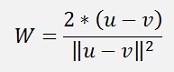
and
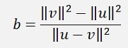
(Please note. In the later described SMO algorithm both will be calculated in a different way)
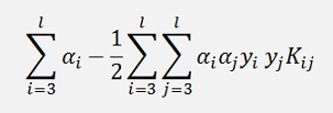
For a numerical solution of the above optimisation problem Lagrange multipliers are introduced. One Lagrange multiplier is add to each data sample and with this the so called Lagrangian is built:
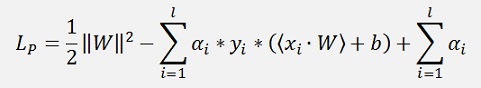
(With l = number of data points and αi the Lagrange multiplier)
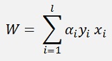
This LP must be minimized. Therefore the gradient of LP with respect to W and b should vanish.
That leads to:
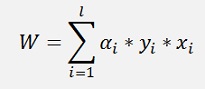
and
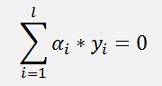
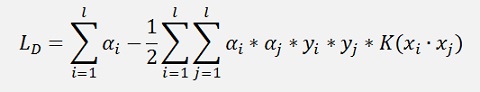
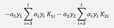
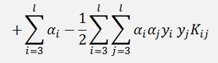
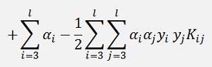
These two constraints can be substituted into the above formula and we get
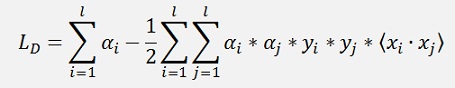
(This function is called the objective function in many articles)
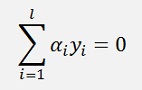
Now the optimisation direction has changed. LD must be maximised and the constraint
Must be fulfilled.
For this maximisation the Lagrange multipliers must be determined. That’s quite a demanding task as there is one Lagrange multiplier for each data point.
At the end of this maximisation many of the Lagrange multipliers will become 0 and the ones that remain >0 are called the support vectors. With these support vectors W and b will be computed.
The sequential minimal optimization by John C. Platt is the fasted algorithm to solve such a problem. It does not optimize all Lagrange multipliers at once. In a loop it runs through all samples and picks just 2 multipliers at a time. These two multipliers can be optimized analytical and this loop is repeated till all multipliers are optimized. Starting from the formulation
I first have to introduce the so called Kernel function
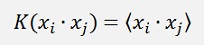
which is the dot product for the moment.
and with
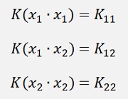
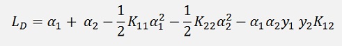
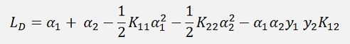
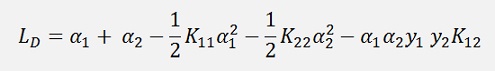
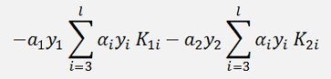
The above formula for just two Lagrange multipliers α1 and α2 can be written as:
As a temporary simplification:
with
we can say
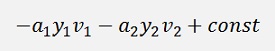
and as the expression
is constant regarding α1 and α2, it can be said
and as
we can say
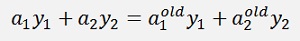
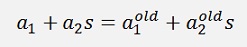
After recalculation of α1 and α2 this equation regarding the values from before the recalculation, with the old values, must remain valid.
Or as y1 and y2 both are 1 or -1 it is as well
With the substitution s = y1*y2
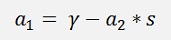
This inserted in the above formulation to eliminate α1:
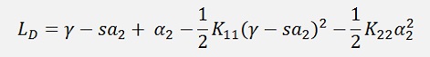
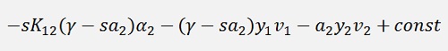
and a little transformed:
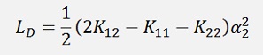
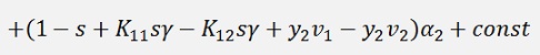
Now the derivation of this should vanish:
or

If the entire expression is multiplied by y2

(Remark that y2 * y2 = 1)
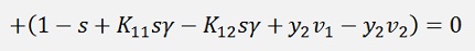
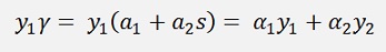
Now, an important step:
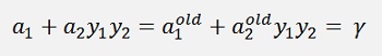
If we look at the substitution of further above 2
This expression is valid for old values from the last iteration to and the equation for γ from further above
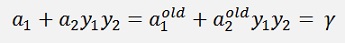
holds for old values as well. That means if we substitute these two formulations into our main formula, we get the new α2 on the left side and on the right side there are all old values
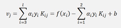
And with
and
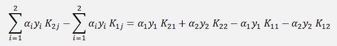
substituted into the above equation:


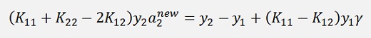
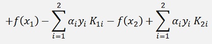
A bit transformed and shortened:

(Remark: K21 = K12. Explanation follows further down)
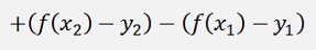
Or the final formulation:
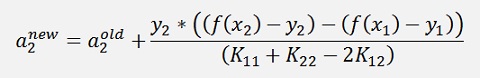
(Remark: I divided the whole expression by y2. But as y2 is 1 or -1 it can as well be multiplied by the fraction). The function values f(x2) and f(x1) are both old values as mentioned further above.
There is one more value that is used all over:
The error value
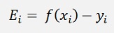
With this
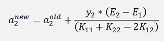
Now there is one more thing:
An approach like this can get problems if the data samples to optimize the function underlay some noise and the two classes overlap each other. For such cases a so called soft margin hyperplane is computed. Therefor the basic function is modified to
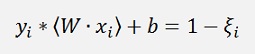
With ξi >= 0.
For this the αi values must be limited as as (and ξi will not appear in the further formulations)
with C as a value between 0 and 1.
There are two cases now:
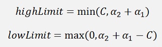
If y1 = y2
If y1 ≠ y2
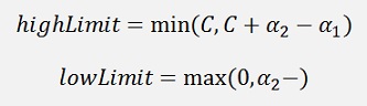
The new α2 must be limited to these boundaries.
After that α1 can be determined by
or
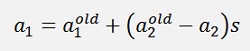
Still with s = y1*y2
Now there is still another thing:
The formulation for α2 only works if
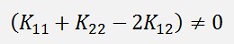
If this is not the case (that can happen if two samples are equal)Platt says the objective function LD
Should be evaluated at each end of the limit and if the function at the lower limit is smaller than the one at the higher limit α2 shall be set to the lower limit and vice versa.
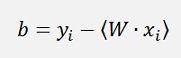
Finally W and b should be computed. If no Kernel is used (explanation follows) W could be computed as
And
For just some i.
But that will most often not be the case (that no Kernel is used).
With a Kernel in use W will not be needed and b is computed as follows:
If α1 is not at its bounds:
and
If α1 is at its bounds but α2 is not at its bounds:
and
If α1 and α2 both are at their bounds:
Like this the entire function to compute α1 and α2 is:
private int ComputeA1A2(int iA1, int iA2)
{
int i, j;
double lLim;
double hLim;
double eta;
double[] x1 = data.values.ElementAt(iA1).x;
double[] x2 = data.values.ElementAt(iA2).x;
double y1 = data.values.ElementAt(iA1).y;
double y2 = data.values.ElementAt(iA2).y;
double a1 = data.values.ElementAt(iA1).a;
double a2 = data.values.ElementAt(iA2).a;
double e1 = data.values.ElementAt(iA1).e;
double e2 = data.values.ElementAt(iA2).e;
double k11, k12, k22;
double s = y1 * y2;
double lObj, hObj;
// limits for a2
if (y1 != y2)
{
lLim = a2 - a1;
if (lLim < 0)
lLim = 0;
hLim = c + a2 - a1;
if (hLim > c)
hLim = c;
}
else
{
lLim = a2 + a1 - c;
if (lLim < 0)
lLim = 0;
hLim = a2 + a1;
if (hLim > c)
hLim = c;
}
if (hLim == lLim)
return 0;
k11 = K(x1, x1);
k12 = K(x1, x2);
k22 = K(x2, x2);
eta = k11 + k22 - 2 * k12;
// calculate a2
if (eta > 0)
{
a2 = data.values.ElementAt(iA2).a + y2 * (e1 - e2) / eta;
if (a2 > hLim)
a2 = hLim;
else
{
if (a2 < lLim)
a2 = lLim;
}
}
else
{
double f1 = y1 * (e1 - b) - a1 * k11 - s * a2 * k12;
double f2 = y2 * (e2 - b) - s * a1 * k12 - a2 * k22;
double l1 = a1 + s * (a2 - lLim);
double h1 = a1 + s * (a2 - hLim);
lObj = l1 * f1 + lLim * f2 + l1 * l1 * k11 / 2 + lLim * lLim * k22 / 2 + s * lLim * l1 * k12;
hObj = h1 * f1 + hLim * f2 + h1 * h1 * k11 / 2 + hLim * hLim * k22 / 2 + s * hLim * h1 * k12;
if (lObj < hObj - eps)
a2 = lLim;
else
{
if (lObj > hObj + eps)
a2 = hLim;
}
}
if (Math.Abs(a2 - data.values.ElementAt(iA2).a) < eps * (a2 + data.values.ElementAt(iA2).a + eps))
return 0;
// calculate a1
a1 = data.values.ElementAt(iA1).a + y1 * y2 * (data.values.ElementAt(iA2).a - a2);
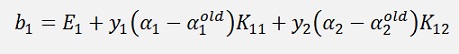
// calculate b
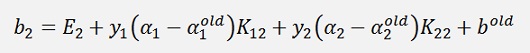
double b1 = e1 + y1 * (a1 - data.values.ElementAt(iA1).a) * k11 + y2 * (a2 - data.values.ElementAt(iA2).a) * k12;
double b2 = e2 + y1 * (a1 - data.values.ElementAt(iA1).a) * k12 + y2 * (a2 - data.values.ElementAt(iA2).a) * k22;
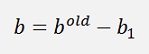
if ((a1 > lLim) && (a1 < hLim))
b = b - b1;
else
{
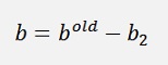
if ((a2 > lLim) && (a2 < hLim))
b = b - b2;
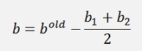
else
b = b - (b1 + b2) / 2;
}
// update values
data.values.ElementAt(iA2).a = a2;
data.values.ElementAt(iA1).a = a1;
// update all error values
for (j = 0; j < samples; j++)
{
double tempU = 0;
for (i = 0; i < samples; i++)
{
tempU = tempU + data.values.ElementAt(i).y * data.values.ElementAt(i).a * K(data.values.ElementAt(i).x, data.values.ElementAt(j).x);
}
data.values.ElementAt(j).e = tempU + b - data.values.ElementAt(j).y;
}
return 1;
}
For the selection which α1 and α2 to optimize at a time, Platt suggests a heuristic that reduces computing time. I just implemented a part of these suggestions. In the very first loop I run through all samples to select a α1 and run through all samples a second time to select a α2. In all other runs I select only α1 samples which have a α1 > 0 and < C. That might take some more time to compute but it looks a bit simpler
My sequence to optimize all Lagrange multipliers looks like:
// Loop to optimize a1 ana a2
while ((numChanged > 0) && (iterationCount < maxRuns))
{
numChanged = 0;
for (i = 0; i < samples; i++)
{
if (firstRun)
{
for (j = 0; j < samples; j++)
{
if (j != i)
numChanged += ComputeA1A2(i, j);
}
}
else
{
if ((data.values.ElementAt(i).a > 0) && (data.values.ElementAt(i).a < c))
{
for (j = 0; j < samples; j++)
{
if (j != i)
numChanged += ComputeA1A2(i, j);
}
}
}
}
firstRun = false;
iterationCount++;
}
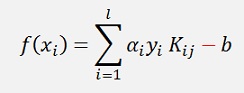
It repeats until it finds no more Lagrange multiplier to be optimized or the maximum number of runs is reached. Then it finishes and all output values are computed by
and displayed.
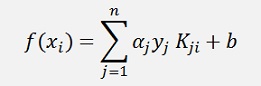
(Remark: f(x) is not computed by the use of W. More to that further down)
In case the data cannot be separated by a hyperplane because the separating border is bent, this case is called linear not separable. To be able to solve such cases as well the so called Kernel trick was invented.
In the objective function
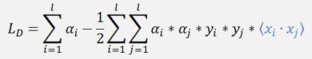
There is a dot product on the right side. This dot product can be replaced by a so called Kernel function. This Kernel function virtually bends the separating hyperplane.
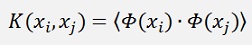
The Kernel function must obey some constraints. The dot product basically transforms the input data into another space: The feature space. And it converts it to a single value. The Kernel function must do the same. So it must have the form
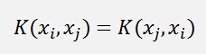
It must be separable into two transformations Φ(x) which is computed in a dot product. That causes the Kernel function to be symmetric. That means
There are many different Kernel functions available to solve different problems and not every Kernel solves every problem.
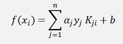
An important fact is, that by the use of a Kernel function the vector W is not needed anymore. Or better to say it’s almost impossible to use it. As we would have to use the transformation
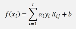
To compute f(x) and Φ (x) is not given in all cases. With a Kernel the output value f(x) must be computed with:
I know there is much more to say about Kernel functions. But I want to keep things short and easy. Therefore I leave that
For the interested reader the book “Learning with Kernels” from Bernhard Schölkopf and Alexander J. Smola might be recommended. But be warned: It’s dry as hardtack
I implemented following Kernels in my sample project:
Polynomial Kernel
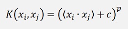
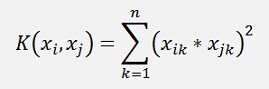
Square dot product Kernel
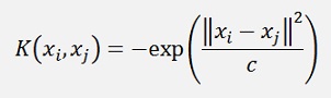
RBF Kernel
This Kernel function must be assigned to the delegate K in the sample project in the constructor like:
K = RBF_Kernel;
With
public delegate double function(double[] x1, double[] x2);
public
function K;
In my sample project I got the best results with the RBF (radial basis function) Kernel.
Sample project with Iris data set
In my sample project I use the Iris data set for classification. The Iris data set contains characteristic data of 150 Iris flowers:
1. sepal length in cm
2. sepal width in cm
3. petal length in cm
4. petal width in cm
5. class:
There are 3 different flowers that should be classified. I did this classification in two steps. First I classify all samples into the 2 classes “Iris Setosa” or not. That gives a first parameter set which is saved in a .Json file that contains 10 support vectors ,W and b. In a second step I use just the data samples of “Iris Versicolour” and “Iris Virginica” and classify these two classes. That gives the second parameter set which contains 38 support vectors, W and b and is saved into a .Json file to. There can be quite some support vectors that have to be transferred to the test application. Therefore I handle this data transfer by .Json files here. The first classification could be done without using a Kernel function. It’s possible to separate this data linear. But as I want to use the same setting for both steps I use the RBF Kernel for both. By the way: In the test application the same Kernel function must be used as it has been used for training.
The data is held in the .Csv files “Data_1.csv” for the first step and “Data_2.csv” for the second step. Which one is loaded is hard coded in the constructor of the Main Window. The data is loaded into the collection
public Collection<TElement> values
In the data class.
There is a constant
const int features_in = 4;
This is the number of features, or dimensions of the input data. This value must fit to the loaded input data.
The member variable
int samples
contains the number of data samples. This value is set automatically after loading the data.
The procedure is to load the first data file, compute the parameters, the application saves these in the file “Trained.Json” in the bin directory. This file must be renamed in “Trained_1.Json”. Then the second file must be loaded (by uncommenting the code line) and the same procedure is done for the file “Trained_2.Json”. The two .Json files must be copied to the test application and this test application is run with the test data. For training I removed the last 5 samples of each flower in the data. So I use only 135 samples for training. The removed 15 samples I use for testing and the application recognises all of them correct. O.k. 15 test samples are not too much. But that’s still better than nothing at all
The main window of the training application looks like:
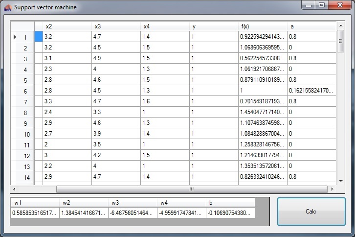
In the upper grid the input data is displayed on the left side. The column “f(x)” displays the classifier value f(x) which is calculated after training and the column “a” shows the Lagrange multiplier of each data sample. In the lower grid the parameters W and b are displayed even if W is not used right now.
When the second step is trained it can be seen that one sample is classified wrong after training. That can be. Possibly it could be avoided if a more sophisticated Kernel would be used. But as all test samples are classified correct I think it’s quite o.k.
One last annotation: John C. Platt uses in his documentation the formulation
While in all the other articles about SVM I saw
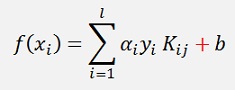
I used this formulation here. That’s why some of my descriptions look a little different from Platt’s descriptions.
For comparison it could be interesting to see
Logistic Regression with the sigmoid function
Backpropagation
As there the Iris data set is processed in different algorithms.