

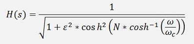
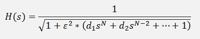
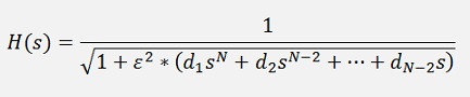
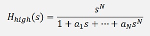
There are 2 types of Chebychev filters: Type 1 (the one that is covered in this article) is a filter type that allows some ripple ε in the pass band and therefore reaches a very steep slope towards the stop band. The transfer function of a Chebychev low pass filter of 4. Order looks like:
(Type 2 is the filter type that has some ripple in the stop band)
This steep slope is achieved by the transfer function
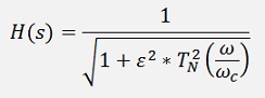
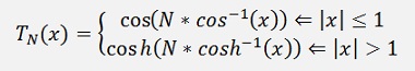
With TN(x) as a Chebyshev polynomial (see Integration by the use of Legendre or Chebychev polynomials) and ε as the ripple factor.
The Chebychev polynomial can be expressed as
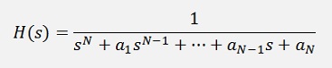
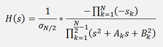
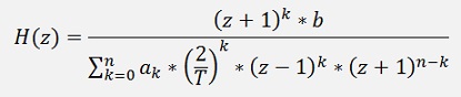
Now, to implement a digital filter the above formulation must be transformed into a form like:
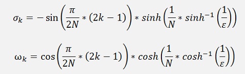
And therefore Chebychev first calculates the poles of his transfer function
They are there where
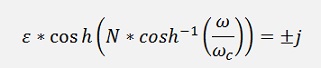
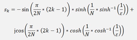
This is a complex equation and it has the solution
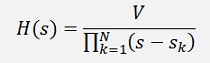
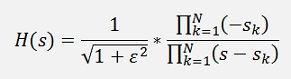
And with this the transfer function becomes
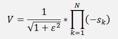
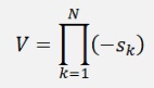
With V as an amplification vactor that has to be determined as next step. To do this we have to distinguish between the cases N is odd and N is even.
If N is even and we insert the Chebychev polynomial of an even order we get the transfer function
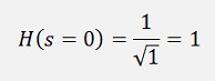
If s = 0 this equation is
But the transfer function we got with our poles gives for s = 0
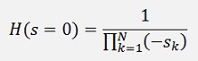
That means V must be
If N is even.
If N is odd we have
And if s = 0
And so
So, if N is even the final transfer function becomes
and if N is odd
This part with the amplification is often missing in the literature. There they describe an algorithm which is not really correct and finally feed everything into MATLAB…And MATLAB just solves the problem

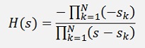
In the literature there is often a form like
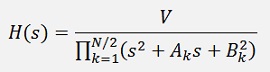
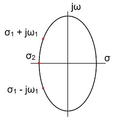
Used for the transfer function. That comes from the fact that the poles are always conjugate complex. The poles are lying on the left side of an ellipse like
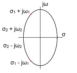
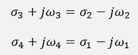
and we always have conjugate complex pairs. Her for instance for N = 4
and these pairs are multiplied together like
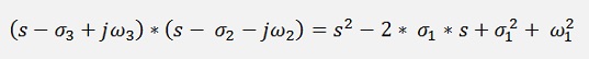
and so
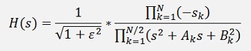
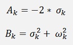
If N is odd we get a little different situation like
One pole is pure real here and we get
and
For both even N and odd N.
This finally implemented in a c# function is
public void CalcChebychev(int order, double t)
{
int i = 1;
double[] poly = new double[3];
double[] poly2 = new double[2];
double nu = Math.Log(1.0 / e + Math.Sqrt(1.0 / e * e + 1.0)) / order;
double sigma;
double omega;
a_s = new double[1];
a_s[0] = 1.0;
b_s = 1.0;
// The denominator of the transfer function
if (order % 2 == 0)
{
poly[0] = 1.0;
for (i = 0; i < order / 2; i++)
{
sigma = Math.Sinh(nu) * Math.Sin(Math.PI * (2.0 * i + 1.0) / 2.0 / order);
omega = Math.Cosh(nu) * Math.Cos(Math.PI * (2.0 * i + 1.0) / 2.0 / order);
poly[1] = 2.0 * sigma;
poly[2] = sigma * sigma + omega * omega;
a_s = Poly.Mult(a_s, poly);
// the enumerator part
b_s = b_s * sigma * sigma + omega * omega;
}
}
else
{
poly[0] = 1.0;
for (i = 0; i < (order + 1) / 2; i++)
{
sigma = -Math.Sinh(nu) * Math.Sin(Math.PI * (2.0 * i + 1.0) / 2.0 / order);
omega = Math.Cosh(nu) * Math.Cos(Math.PI * (2.0 * i + 1.0) / 2.0 / order);
if (i < (order) / 2)
{
poly[1] = -2.0 * sigma;
poly[2] = sigma * sigma + omega * omega;
a_s = Poly.Mult(a_s, poly);
// the enumerator part
b_s = b_s * sigma * sigma + omega * omega;
}
else
{
poly2[0] = 1;
poly2[1] = -sigma;
a_s = Poly.Mult(a_s, poly2);
// the enumerator part
b_s = b_s * sigma;
}
}
}
// the amplification in the enumerator
if (order % 2 == 0)
b_s = -b_s * Math.Sqrt(1.0 + e * e);
else
b_s = -b_s;
}
This function calculates the transfer function in the Laplace domain and puts it into the array a_s for the denominator and into the double value b_s for the enumerator. An important fact is here that these parameters are independent on any frequency. Here only the ripple ε and the order N of the Chebychev polynomial matter. The frequencies get into the scene when the transfer function is transformed into the z domain.
This transformation into the z domain is done the same way I did it in Digital filter design, by a bilinear transformation with
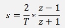
and
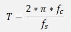
with fc = cut off frequency of the filter and fs = sampling frequency.
The transfer function in the z domain becomes
with fc = cut off frequency of the filter and fs = sampling frequency.
The function to transform is more or less the same as I used it in the Bessel filter . Only the initialisation of the enumerator is a bit different as the input is not just 1 for this.
public void TransformToZPlane()
{
int i, j;
List<double[]> aa = new List<double[]>();
for (i = 0; i <= order; i++)
{
aa.Add(new double[] { 1.0, -1.0 });
}
double[] tempA = { 1.0, 1.0 };
tempA[0] = 1;
tempA[1] = 1;
b_z = Poly.Power(tempA, order);
b_z = Poly.Mult(b_z, b_s);
tempA[1] = 1;
for (i = 0; i <= order; i++)
{
double[] tempEl = aa.ElementAt(i);
tempEl = Poly.Mult(Poly.Power(tempA, i), Poly.Power(tempEl, order - i));
tempEl = Poly.Mult(tempEl, a_s[i] * Math.Pow(2.0 / tc, order - i));
aa.RemoveAt(i);
aa.Insert(i, tempEl);
}
for (i = 0; i <= order; i++)
{
a_z[i] = 0;
for (j = 0; j <= order; j++)
a_z[i] = a_z[i] + aa.ElementAt(j)[i];
}
for (i =0; i < b_z.Length; i++)
{
b_z[i] = b_z[i] / a_z[0];
}
for (i = a_z.Length-1; i >= 0; i--)
{
a_z[i] = a_z[i] / a_z[0];
}
}
I initialize the filter like:
t = 2.0 * Math.PI * fc / fs;
TChebychev cheb = new TChebychev(order, t, 0.2);
cheb.CalcChebychev(order, t);
cheb.TransformToZPlane();
For a ripple of 0.2 dB and get the denominator and enumerator polynomial in
cheb.a_z;
cheb.b_z;
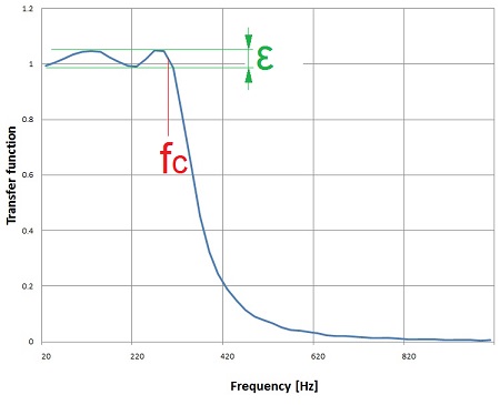
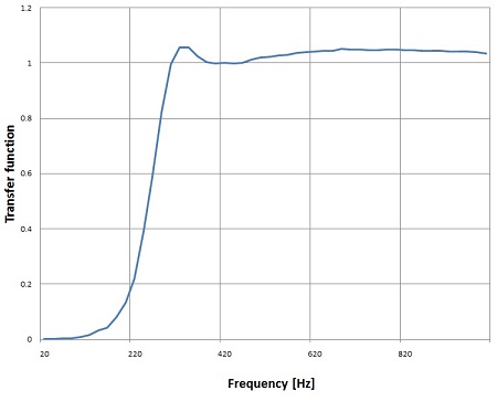
With these parameters I get with fs = 10 kHz and fc = 300 Hz and order = 4 the transfer functionn
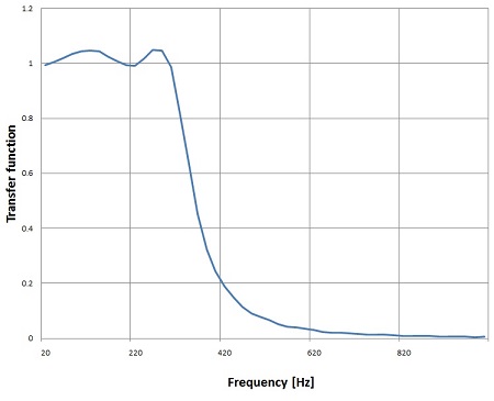
It has a really steep slope. That looks quite cool. With higher order it get’s even steeper. But the higher the order the more critical the ripple becomes. The Chebychev filter is quite sensitive on too big ripples. If the order is bigger than 4 the ripple should be smaller than 0.1 dB else the algorithm goes crazy
High pass filter
The transformation of the low pass filter into a high pass filter is done by a so called low-pass to high-pass transformation. That just means to replace s by 1/s in the transfer function like
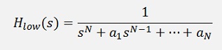
That is
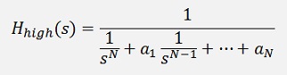
or without compound fraction
In the implementation that means I just have to switch the direction of the elements of my denominator polynomial and add the SN in the enumerator. This can be done in the transformation from Laplace to z domain.
public void TransformToZPlane(bool bHighPass)
{
int i, j;
double[] tempA = { 1.0, 1.0 };
tempA[0] = 1;
if (bHighPass)
{
tempA[1] = -1;
b_z = Poly.Power(tempA, order);
b_z = Poly.Mult(b_z, Math.Pow(2.0 / tc, order));
double[] temp = new double[a_z.Length];
for (i = 0; i < a_s.Length; i++)
temp[i] = a_s[a_s.Length - 1 - i];
for (i = 0; i < a_s.Length; i++)
a_s[i] = temp[i];
}
else
{
tempA[1] = 1;
b_z = Poly.Power(tempA, order);
}
b_z = Poly.Mult(b_z, b_s);
tempA[1] = 1;
With this small modification the filter can work as high pass filter as well and shows a transfer function
That’s it
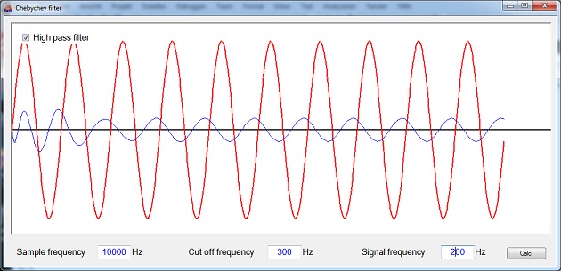
The demo project consists of one main window. It processes a short sample signal (red curve) and displays the filtered signal (blue curve) the cut off frequency, sampling frequency and signal frequency can be set and in the left upper corner of the graphic is a checkbox where high or low pass behaviour can be selected.
A online solver in JavaScript, that returns the filter parameters, can be found on Chebychev filter