

There are many descriptions about the second order Goertzel algorithm to be found in the net. But most of them do not explain its derivation in fully. There is always the same part missing. So I try to fill this gap

The second order Goertzel algorithm is an advancement of the first order Goertzel algorithm
(for the entire description see first order Goertzel algorithm)
it is used to perform a Discrete Fourier Transformation and it’s quite a bit faster than the basic DFT algorithm. But it is less accurate and can be unstable in certain cases. But let’s start with the first order Goertzel algorithm first.
The first order Goertzel algorithm has the following simple form
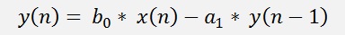
For n = 1 to N
In the digital signal processing this formula corresponds to the signal path
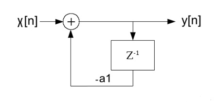
and the transfer function
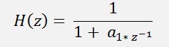
with
Now the big issue here is the complex denominator in the transfer function. To simplify the transfer function Goertzel multiplyied the enumerator and denominator by 1 + the conjugate of a1 * z^-1. That makes the denominator a real value and leads to:
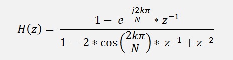
And this corresponds to the difference equation
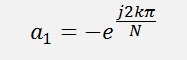
with the substitution
For a long time I was wondering why they are doing this. The difference equation looks much more complicate now. But there is some advantage at the end
Here most of the explanations now say: “As we are only interested in c[n], we can leave the complex multiplication b1 * y[n-1] till the end of the calculation and have to carry it out only once at the end”… That’s not the whole truth. We are interested in c[n] and the complex calculation can be put to the end of the calculations. But there is no relation between this two things. It took me a deep look into the theories of digital signal processing to find out why
The big step lays in the signal path. The signal path to the difference equation further above looks like:
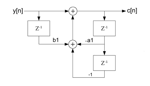
If we would implement this. It would be something like
put into a loop. In each cycle we had the complex multiplication b1 * x[n-1] and due to that the whole calculation had to be carried out complex. Much more calculation effort than required in the first order Goertzel algorithm. That’s not what we want.
But the signal path can as well be drawn like this:
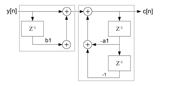
Now we have two independent transfer functions and these two functions can be switched without influencing the resulting transfer function.
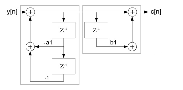
And we even can put them together again. This form is called the direct form II of the signal path and looks much better. The feedback part is now at the beginning of the function.
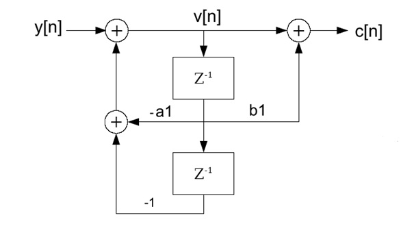
This put into code we get
for the left feedback part and
For the right feed forward part.
and still
The feedback part has to be implemented in a loop running through all the samples of y. That means from 0 to N-1.
for
(n = 0; n < N; n++)
{
v0.real
=
y[n].real - a1.real * v1.real - v2.real;
v2
= v1;
v1
= v0;
}
I used complex data types because at the end we have complex numbers.
The right part needs to be calculated only once at the end of the calculation (and it has nothing to do with the fact that we are looking for c[n] only
. Basically the right part contains the complex
multiplication v[n-1] * b1. So far we only had
real values to deal
with. That means v[n-1] is real and has no imaginary part. Therefore
the following complex multiplication becomes not very complicate. The
real part becomes v[n-1]. real * b1.real and the imaginary part becomes
v[n-1].real * b1.imag. Finally we are looking for the Fourier
componentsBoth values should be calculated as
Now for the real part that’s
As v[n] is a real value and has no imaginary part. The calculation for the imaginary part c[k].imag becomes a bit shorter:
And finally both values have to be divided by N because of
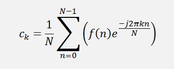
With this the sequence for all the Fourier components a[0] to a[N-1] and b[0] to b[N-1] is:
for (k = 0; k < N;
k++)
{
v0.real = 0;
v0.imag = 0;
v1.real = y[1].real;
v1.imag = y[1].imag;
v2.real = y[0].real;
v2.imag = y[0].imag;
b1.real = -Math.Cos((double)(2.0 * Math.PI
* (double)(k) / (double)(N)));
b1.imag = Math.Sin((double)(2.0 * Math.PI
* (double)(k) / (double)(N)));
a1.real = -2 * Math.Cos((double)(2.0 * Math.PI
* (double)(k) / (double)(N)));
a1.imag = 0;
for (n = 0; n < N; n++)
{
v0.real = y[n].real - a1.real * v1.real -
v2.real;
v2 = v1;
v1 = v0;
}
c[k].real = (v0.real + b1.real * v2.real) / (double)(N)
* 2.0;
c[k].imag = -(b1.imag * v1.real) / (double)(N)
* 2.0;
}
Implemented like this the second order Goertzel algorithm is a very fast way to carry out a Discrete Fourier transformation. On my computer the test application with 1000 samples takes 8 ms. A standard implementation of the Discrete Fourier transformation takes 120 ms for the same calculation. But this increase of calculation speed costs some accuracy and the Goertzel algorithm is not stable in any case. Already in my test application some inaccuracy is visible. For the rectangle signal all the real parts should become 0. But a[1] = -0.12, a[2] = 0.04, a[3] = -0.11 and so on. In the standard implementation a[1] = 0.04, a[2] = 0.04, a[3] = 0.04 for the phase shift of the harmonics that can make quite a difference.
The second order Goertzel algorithm is a very quick thing but it has its disadvantages. I made a bit a quicker implementation of the Discrete Fourier transformation by putting the calculations of all the used exp(j2kπ/N) values into an array and picking them from there. With this algorithm the same transformation runs in 20 ms and is as accurate as the standard implementation. See
that could be a good alternative
For the analytic Fourier transformation of the used sample signals see Fourier transformation