

Basically
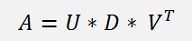
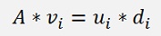
The singular value decomposition (SVD) of a matrix A is a factorisation of this matrix into the product of 3 matrixes UDV according to
U and V (the transposed of V is used in the equation) are both orthonormal matrixes and D is a diagonal matrix containing positive real values. The columns of U are called the left singular vectors and the columns of V are the right singular vectors. The diagonal values of D are the singular values.The decomposition is defined for n*m matrixes where n >= m (n is the number of rows and m the number of columns). That means A can be square or higher than wide. In most documentations they say the size of U is n * r, D is r * r and V is m * r with r as the rank of A (I don’t agree with that). Some say D is n * n (that’s much better). I say U is n * n, D is n * m and V is m * m. Otherwise the multiplication U * D * VT will never give A which has the size of n * m. But more to this later

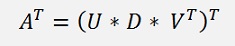
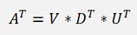
For the singular value decomposition of a square and regular matrix the first step is to compute D and V. For the derivation we use the equation
If this entire equation is transposed:
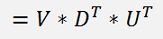
the right side can be transformed like
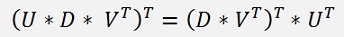
(See Transposed Matrix for an introducition to Transposed Matrixes)
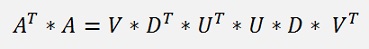
this and the origin equation composed:
and with
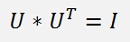
this part can be kicked out and the equation looks like:
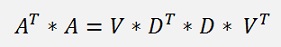
Both sides extended by V on the right side VT * V can also be kicked out:
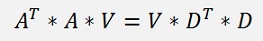
Now we substitute DT * D = L.
L is a diagonal matrix containing the squares of the dii elements.
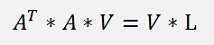
Now there is an interesting step: If we look at just one column vector vi of V now, the equation becomes:
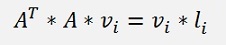
For i = 1 to m
Note: li is a single number and hence this is the equation for one Eigenvalue li and its Eigenvector vi of the matrix AT * A. That means to compute D and V we have to multiply AT by A and compute the Eigenvalues and Eigenvectors of this. The diagonal elements of D are the square roots of the Eigenvalues and the column vectors of V are the Eigenvectors of AT * A.
The result of AT * A is a symmetrical matrix and the Eigenvalues of this symmertical matrix can be computed by the use of Jacobi transformations (See Eigenvalues of a symmetric matrix by Jacobi for details) . That makes the computation quite simple and we get the Eigenvalues and Eigenvectors at once. We just have to initialise V by setting it up as a unit matrix I and run the Jacobi transformation in an iterative loop till we get the Eigenvalues and multiply V each cycle by the Jacobi rotation matrix. That can be done in a short function:
public void RunJacobi(int maxOrder)
{
int
i, k, count = 0;
double delta = 10;
while ((delta > 1.0E-100) && (count < 50))
{
}double delta = 10;
while ((delta > 1.0E-100) && (count < 50))
{
delta
=
0;
count++;
for (i = 0; i < maxOrder; i++)
{
}count++;
for (i = 0; i < maxOrder; i++)
{
for
(k = i + 1; k < maxOrder; k++)
{
if(i< maxOrder-1)
delta = delta + Math.Abs(a[i+1, i]);
}{
if
(a[k, i] != 0.0)
{
}{
CalcRMatrix(a,
i, k, maxOrder);
a = Matrix.MultTranspMatrixLeft(a, r, i, k, maxOrder);
a = Matrix.MultMatrixRight(a, r, i, k, maxOrder);
v = Matrix.MultMatrixRight(v, r, i, k, maxOrder);
}a = Matrix.MultTranspMatrixLeft(a, r, i, k, maxOrder);
a = Matrix.MultMatrixRight(a, r, i, k, maxOrder);
v = Matrix.MultMatrixRight(v, r, i, k, maxOrder);
if(i< maxOrder-1)
delta = delta + Math.Abs(a[i+1, i]);
with
double[,] a = new double[n, n];
double[,] r = new double[n, n];
double[,] v = new double[n, n];
and the rotation matrix like
public void CalcRMatrix(double[,] a, int p, int q, int size)
{
int i, j;
double phi;
double t;
phi = (a[q, q] - a[p, p]) / 2 / a[q, p];
if (phi != 0)
{
if (phi > 0)
t = 1/(phi + Math.Sqrt(phi * phi + 1.0));
else
t = 1/(phi - Math.Sqrt(phi * phi + 1.0));
}
else
t = 1.0;
for (i = 0; i < size; i++)
{
for (j = 0; j < size; j++)
{
r[i, j] = 0.0;
}
r[i, i] = 1.0;
}
r[p, p] = 1 / Math.Sqrt(t * t + 1.0);
r[p, q] = t * r[p, p];
r[q, q] = r[p, p];
r[q, p] = -r[p, q];
}
After running the function RunJacobi the Eigenvalues will be in the diagonal elements of the matrix a. We take the square root of them and order them in descending order. The only, but important thing to consider is to do the same ordering with V as the columns of V belong to the columns of D
With this we can compute U and that starts with the origin equation again.
Both sides extended by V and VT * V kicked out on the right side:
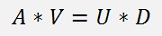
If we write this equation for just one column vector:
Where di is one single number and i runs from 1 to m.
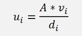
This can be resolved for ui.
And for one element of the vector ui:
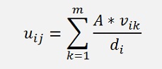
With j = 1 to n.
In code that’s:
for (i = 0; i < rank; i++)
{
for (j = 0; j < OrderY; j++)
{
u[j, i] = 0;
for (k = 0; k < OrderX; k++)
{
u[j, i] = u[j, i] + ori[j, k] * v[k, i];
}
if(d[i] != 0)
u[j, i] = u[j, i] / d[i];
}
}
Now there is a first special case: The outer loop runs only to the Rank of the matrix A instead of m. If the matrix A is not regular and has some columns depending on each other, we will not get all diagonal elements of D set. The columns of U can only be computed for the diagonal elements of D which are not 0. But as this chapter describes the computation of the singular value decomposition of regular matrixes, we are done for this
Singular value decomposition of a matrix of lower rank
If the rank of a matrix is smaller than its number of rows that means there are some columns dependant on each other or the matrix is higher than wide. If the matrix A is higher than wide, the product AT * A will be square and the size will be equal to the number of columns A has. Therefore the size of D will be smaller than the size of A. If A is a square matrix but its rank is smaller than its number of rows, not all diagonal element of D will be set and some will be 0. In both cases we cannot complete all columns of U with the above sequence. To finish the calculation of the u elements in this case we first have to determine the Rank of matrix A which is the index of the last diagonal element of D that is not 0 (the values must be sorted the biggest first). The empty columns must be filled by vectors that are orthogonal to the column vectors determined so far. If we would compute the SVD of a 6 * 6 matrix with the rank = 4, the first 4 rows of U would be filled by the above sequence and we would have to find one vector for column 5 that is orthogonal to the first 4 column vectors and a second vector for column 6 that must be orthogonal to the first 4 and the 5th to.
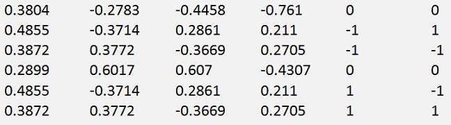
In my sample matrix
the computed rows of U look like
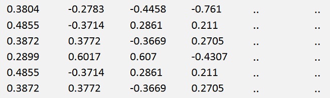
It’s a 6 * 6 matrix with the rank = 4 and the last 2 columns are empty. To find a vector that is orthogonal to the first column vector the scalar product of this vector u1 and the searched vector u5 must be 0. That means
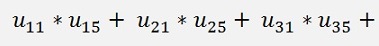
The same must be valid for all 4 column vectors.
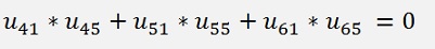
That leads to the matrix equation
This matrix equation can be solved by a little modified Gaussian elimination algorithm (See The elimination algorithm by Gauss) . While eliminating the elements below the main diagonal there is the special case that, in case of dependant rows in U we get dependant columns here. In such a dependant column all elements except the first on become 0 by the elimination function .To avoid divisions by cero I implemented a function SwitchRows(int n) to be used if the actual used diagonal element is 0 my implementation of the Gaussian elimination algorithm. This function does not help here and I replaced it by the function SwitchColumns(int n) and call this function if the diagonal element is 0. That moves the column to the very righ fo the matrix where the free elements are. There it does not bother anymore (o.k. I say if the diagonal element is 0 the chances that all other elements in the row are o to are quite high). But as we are switching columns now we have to take care to reorder these columns at the end. Otherwise the elements of the solution vector will have the wrong order. Therefore the origin index of each column is saved in the array index and after solving the matrix equation the function Reorder() uses this index to get the solution vector into the correct order again.
After building the diagonal matrix by elimination of the lower elements we will have 0 values in the last 2 rows and that means the last two elements of u5 are free. So I set them to 1 and compute the others with this.
The same I do for the last column vector and get the following U matrix
This procedure is carried out in a function:
void FillCols(int empties)
{
int
i, j;
int index;
TGauss Gauss = new TGauss(OrderY);
for (index = 0; index < empties; index++)
{
}int index;
TGauss Gauss = new TGauss(OrderY);
for (index = 0; index < empties; index++)
{
for
(i = 0; i < OrderY; i++)
{
Gauss.Eliminate();
Gauss.Solve(empties - index);
for (i = 0; i < Gauss.order; i++)
{
}{
for
(j = 0; j < OrderY; j++)
{
Gauss.y[i] = 0;
}{
Gauss.a[j,
i] = u[i, j];
}Gauss.y[i] = 0;
Gauss.Eliminate();
Gauss.Solve(empties - index);
for (i = 0; i < Gauss.order; i++)
{
u[i,
OrderY - empties + index] = Gauss.x[i];
}with the elimination function
public bool Eliminate(int empties)
{
int
i, k,
l;
bool calcError = false;
i = 1;
for (l = 0; l < order; l++)
{
for (k = 0; k <= order - 1 - empties; k++)
{
return !calcError;
}bool calcError = false;
i = 1;
for (l = 0; l < order; l++)
{
index[l]
= l;
x[l] = 0.0;
y[l] = 0.0;
}x[l] = 0.0;
y[l] = 0.0;
for (k = 0; k <= order - 1 - empties; k++)
{
l
= k + 1;
while ((Math.Abs(a[k, k]) < 1e-8) && (l < order))
{
if (l < order)
{
else
}while ((Math.Abs(a[k, k]) < 1e-8) && (l < order))
{
SwitchColumns(k);
l++;
}l++;
if (l < order)
{
for
(i = k; i <= order - 2; i++)
{
}{
if
(!calcError)
{
}{
if
(Math.Abs(a[i
+ 1, k]) > 1e-8)
{
}{
for
(l = k + 1; l <= order - 1; l++)
{
y[i + 1] = y[i + 1] * a[k, k] - y[k] * a[i + 1, k];
a[i + 1, k] = 0;
}{
a[i + 1, l] = a[i + 1, l] * a[k,
k] - a[k, l] * a[i + 1, k];
}y[i + 1] = y[i + 1] * a[k, k] - y[k] * a[i + 1, k];
a[i + 1, k] = 0;
else
calcError
= true;
return !calcError;
and the solving function
public void Solve(int empties)
{
int
k, l;
for (l = order - 1; l > order - empties - 1; l--)
x[l] = 1.0;
for (k = order - empties - 1; k >= 0; k--)
{
Reorder();
}for (l = order - 1; l > order - empties - 1; l--)
x[l] = 1.0;
for (k = order - empties - 1; k >= 0; k--)
{
for
(l = order - 1; l > k; l--)
{
x[k] = y[k] / a[k, k];
}{
y[k]
=
y[k] - x[l] * a[k, l];
}x[k] = y[k] / a[k, k];
Reorder();
of the class TGauss.
With this we are basically done. The only thing that remains is to check the result by computing A from these found matrixes.
As
We first have to multiply U by D. Now the sizes of the found matrixes become interesting:
If U has the size hu * wu (for height and width) and D has hd * wd, the size of the product U * D will be hu * wd. If this product is multiplied by VT now, the size of this will be hu * hv which should be equal to ha * wa. That means H must be as high as A and as U is square the size of U must be n * n of A. To multiply U * D, D must be as height as U is wide. V is square and as wide and height as A is wide and as U * D must be as width as V, D must be as width as V. S all in all U is n * n, D is n * m and V is m * m. By the calculation of the Eigenvalues the size D is similar to the size of V. That’s no problem as long as n = m. But as soon as m is smaller than n, the size of D must be modified to n * m. That means we have to ad empty rows at the bottom of D. With this modification U * D * VT should give A and if this is the case our calculations were successful
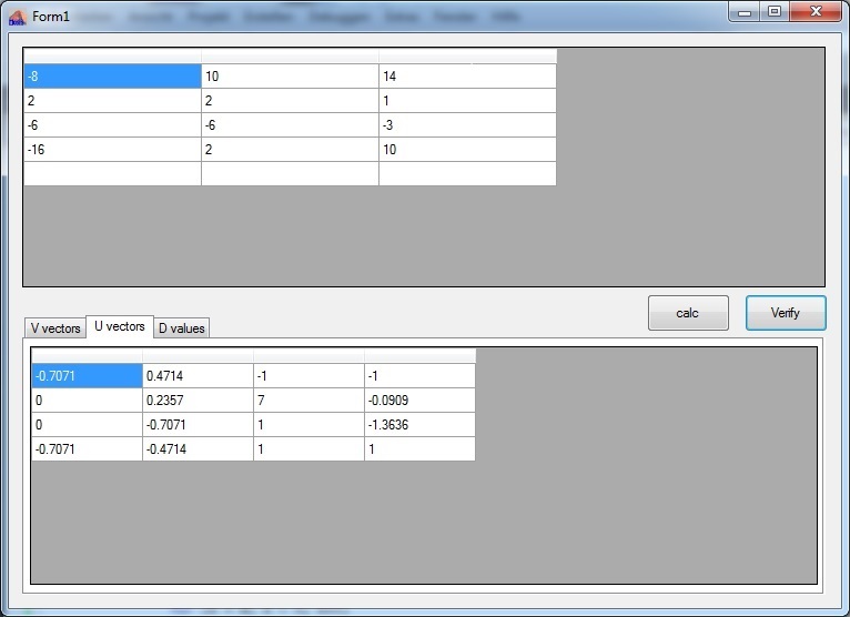
My sample project contains one main window with a grid for A on top and 3 grids in a page control for U, V and D. Pressing "calc" performs the calculation of U, V and D and writes their values in the grids. In the grid of A the values of matrix AT*A after computing the Eigenvalues is written after the calculations of U, V and D. Pressing "verify" carries out U * D * VT and writes the result into the grid of A for checking. All the main calculations are implemented in MainWin.cs. Except the matrix calculations and TGauss are in separate moduls.
Some related articles:
C# Demo Project Singular value decomposition
Java Demo Project Singular value decomposition