

The method of the least squares is a standard procedure to approximate a function like here a polynomial function to a set of reference points if the order of the polynomial is smaller than the number of data points.
There could as well be another function than a polynomial one to approximate. It’s just a matter of setting up the matrix equation and the function for the approximation. I’m using a polynomial function here.
There are several approaches to compute this approximation. Using the singular value decomposition (See Singular value decomposition) is a rather complicate one, but it should (compared with the Method of the least squares ) provide very small deviations to the reference points in some cases. With the polynomial function I have not experienced that so far. But never the less it’s an very interesting algorithm

The method of Cardano is based on the reduction of the equation polynomia

Whereas d is the solution vector containing the y values:
For the deviations additionally the vector r is added. That’s the vector of the residues:
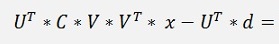
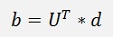
Now both sides are extended by UT from the singular value decomposition:
And as V*VT = I, this can be added on the left side without affecting the equation:

Now there comes a cool step (at least I regard it as that
):
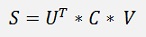
The formulation of the singular value decomposition says
This can be transformed to
(See Transposed matrix)
and so
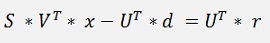
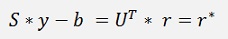
From here there come two substitutions with:
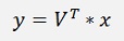
and
And with this
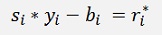
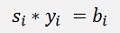
The matrix S is the matrix of the singular values. It is a diagonal matrix containing the singular values in the main diagonal, b is a vector and r* is a vector to. That means the above equation reduced for one single element is:
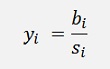
For i = 1 to rank of C (which is basically the order of the polynomial that is searched)
For i > rank si = 0 and therefore
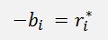
So these elements of the residual vector are given. The deviation of the searched polynomial is the smallest if the length of the vector of the residues is the smallest. As the elements ri for I > rank are already given by –bi = ri. The length of r becomes the smallest if ri = 0 for i= 0 to rank and therefore r*i = 0 and in this case
And now the substitutions are done backward:
And as
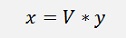
And xi is one of the elements of the searched polynomial.
This backward substitution is done in two loops:
for (i = 0; i < order; i++)
{
b
= 0;
for (j = 0; j < samples; j++)
{
y[i] = b / l[i];
}for (j = 0; j < samples; j++)
{
b
= b + u[j, i] * y_k[j];
}y[i] = b / l[i];
For yi
And
for (i = 0; i < order; i++)
{
x[i]
= 0;
for (j = 0; j < order; j++)
{
}for (j = 0; j < order; j++)
{
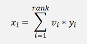
x[i]
=
x[i] + v[i,j] * y[j];
}For xi
Whereas “order” is the order of the searched polynomial and the rank of the matrix C. That looks like a very lean algorithm, but keep in mind, the singular value decomposition has to be carried out before. And that’s still quite a task involving the comoputation of singular values. For a detailed description of this please (See Singular value decomposition)
In my sample application this algorithm creates the following graph
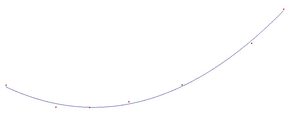
With a polynomial of the order = 3 and the data points
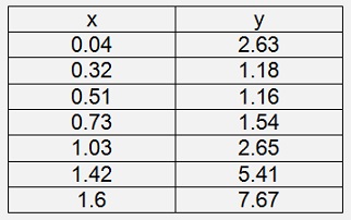
The approximation a3x2 + a2x + a1 polynomial gets the elements
a1 = 2.7492, a2 = -5.9547, a3 = 5.6072
and with these the deviations to the data points is
The order of the polynomial can be increased till 7. Then all the data points are met and we carry out a polynomial interpolation
C# Demo Project Method of the least squares with SVD