

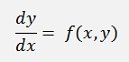
In 1883 John Couch Adams and Francis Bashforth or Forest Ray Moulton developed multistep algorithms to approximate the solution of a differential equation like
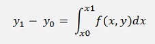
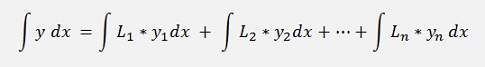
Therefore they integrate both sides of this equation and get
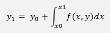
Or resolved for y1:
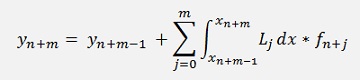
If this formula is written for a y at random position n, it’s
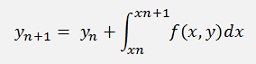
And that’s the basic equation to solve a differential equation in an iterative way. Now, a very simple approach to solve this equation would be to compute the definite integral by a trapezoidal method. But that would be very inaccurate. A better approach is to use Lagrange polynomials same as it is done in the Numerical integration by Newton Cotes algorithm.
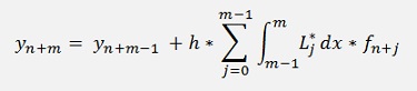
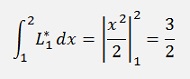
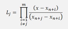
With these Lagrange polynomials the integration looks like:
or
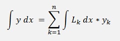
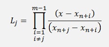
with
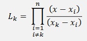
In the Adams algorithms only the las few y values are used to build a polynomial of rather low order. There are two versions of the Adams algorithm: An explicit version that kind of extrapolates yn+1 and an implicit version that includes the yn+1 value to compute the integration.
Explicit method by Adams-Bashforth
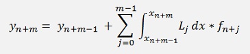
The factors Lj for the Lagrange polynomial are built by the last m-1 data points, excluding the very last one which would be yn+m. For the integration only the interval m-1 till m is used. That’s the part between yn+m-1 and yn+m. That means the function that is given by the Lagrange polynomial is extrapolated in this area. A remarkable detail

As the distance between all xk and xk+1 is constant for all k’s
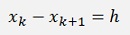
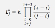
and
With m = order of the Lagrange polynomials.
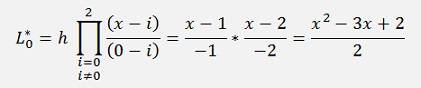
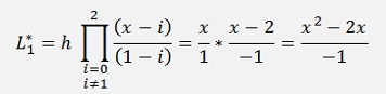
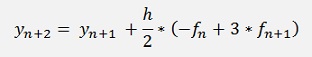
In my sample project I implemented the Adams-Bashforth algorithm with second order Lagrange polynomials.
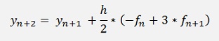
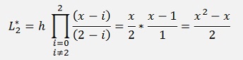
That means:
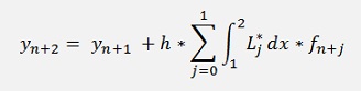
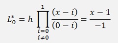
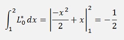
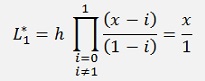
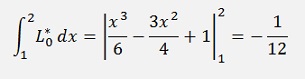
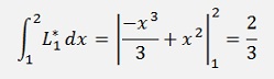
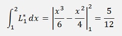
And with this
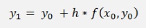
The first two values of y cannot be determined like this. The value of value y0 is defined by the start conditions and y1 can be calculated by a linear extrapolation of the Euler method
A small loop that approximates the function f(x,y) into the arrays xp and yp from where it can be plot into a graph is:
int i;
double h = 3.0 / (double)(datapoints - 1);
xp[0] = 0;
yp[0] = 1; // Start condition
xp[1] = h;
yp[1] = yp[0] + h * f_xy(xp[0], yp[0]);
for (i = 2; i < datapoints; i++)
{
xp[i] = i * h;
yp[i] = yp[i - 1] + h / 2 * (3 * f_xy(xp[i - 1], yp[i - 1]) - f_xy(xp[i-2], yp[i-2]));
}
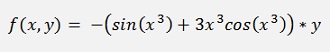
In my sample project I use the equation
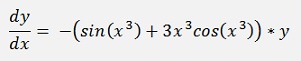
With the start condition y0 = 1
So
double f_xy(double x, double y)
{
return -(Math.Sin(x * x * x) + 3 * x * x * x * Math.Cos(x * x * x)) * y;
}
With x = 3 the exact solution for y is 0. With 1000 sample points I have h = 0.003 and with x = 3, y = 0.06. That’s not too bad. Compared to the 4. order Runge Kutta algorithm that gets 0.056 with 1000 data samples, the Runge Kutta is not much more accurate. Even though it is quite a bit more complicate
Implicit method by Adams-Moulton
Similar to the Adams-Bashforth algorithm the Adams-Moulton algorithm uses the last few y values for the approximation. But it includes the new function value fn+m to. Due to that it finally has to calculate yn+m in a ( most often) not linear equation. That makes things a bit more complicate.
The equation for the Adams-Bashforth algorithm is:
Remark that the sum as well as the product, both are built till m (the Adam-Bashforth goes till m - 1).
That looks not too different from Adam-Bashforth but at the end we will have yn+m on both sides of the equation and have to resolve the equation for this yn+m. That means the function f(x, y) will have to be split somehow and the algorithm cannot be implemented independent on the form of f(x, y). But first we set up a equations for Adams-Moulton with second order Lagrange polynomials.
and with this
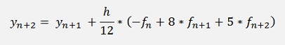
but
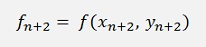
That means yn+2 is on both sides of the equation and we have to resolve the equation for yn+2 (if this is possible). In the sample project with
that’s (fortunately) quite easy and we get
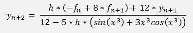
So the loop for this algorithm becomes
int i;
double h = 3.0 / (double)(datapoints - 1);
double fx;
xp[0] = 0;
yp[0] = 1;
xp[1] = h;
yp[1] = 1;
for (i = 2; i < datapoints; i++)
{
xp[i] = i * h;
fx = (Math.Sin(xp[i] * xp[i] * xp[i]) + 3 * xp[i] * xp[i] * xp[i] *
Math.Cos(xp[i] * xp[i] * xp[i]));
yp[i] = (h * (-f_xy(xp[i - 2],
yp[i - 2]) + 8 * f_xy(xp[i - 1], yp[i - 1])) + 12 *yp[i - 1])/(12 + 5 * h *
fx);
}Quite a bit more complicate than the Adams-Bashforth algorithm and it is not that much more accurate. With 1000 sample points it gets at x = 3 an y = 0.057.
To avoid this resolving of f(x,y) the so called predictor corrector method can be applied. That means the Adams-Bashforth method of the same order is used to calculate yn+2 like:
And this is used in
With that the loop would look like:
for (i = 2; i < datapoints; i++)
{
xp[i] = i * h;
fx = yp[i - 1] + h / 2 * (3 * f_xy(xp[i - 1], yp[i - 1]) - f_xy(xp[i - 2], yp[i - 2]));
yp[i] = yp[i - 1] + h / 12 * (-f_xy(xp[i - 2], yp[i - 2]) + 8 * f_xy(xp[i-1], yp[i-1]) + 5 * f_xy(xp[i], fx));
}
With 1000 sample points this one gets y = 0.0561 at x = 3: Even a bit better than the above implementation.
Both algorithms compared to the Runge Kutta algorithm I think the Adams-Moulton algorithm is not too interesting as it is in any way more complex than the Adams-Bashforth algorithm. The Adams-Bashforth is a little bit less accurate as long as it uses the same order polynomial as the Adams-Moulton algorithm does. But if the Adams-Bashforth is implemented with a higher order polynomial, it can even be better than a Runge Kutta algorithm. With a 3. order polynomial the Adams-Bashforth algorithm is:

Now y2 needs to be determined in advance to. That can be done by the usage of a second order Adams-Bashforth formula.
Implemented like this the loop looks like:
int i;
double h = 3.0 / (double)(datapoints - 1);
xp[0] = 0;
yp[0] = 1; // Start condition
xp[1] = h;
yp[1] = yp[0] + h * f_xy(xp[0], yp[0]);
xp[2] = 2 * h;
yp[2] = yp[1] + h / 2 * (3 * f_xy(xp[1], yp[1]) - f_xy(xp[0], yp[0]));
for (i = 3; i < datapoints; i++)
{
xp[i] = i * h;
yp[i] = yp[i - 1] + h / 12 * (5 * f_xy(xp[i - 3], yp[i - 3]) - 16 *
f_xy(xp[i-2], yp[i-2]) + 23 * f_xy(xp[i -
1], yp[i - 1]));
}And this one gets with 1000 sample points for x = 3 an y = 0.055. With a much simpler implementation (and derivation as well) it is even a bit more accurate than a 4. order Runge Kutta algorithm. That’s pretty cool
The reason for this good performance is the fact that, similar to the Runge Kutta algorithm, the Lagrange polynomial interpolate the function and this interpolation is quite good.