

Eric Harold Neville had quite a simple idea to carry out an interpolation between some supporting points.
Starting with just 2 points (x0, y0) and (x1, y1) the idea was to use the value of one supporting point fully on its side and fade it out the closer the interpolation gets to the other point till its weight is 0 at the other point. And do the same with the other point. That means the value of the point on the left side is multiplied by (x1 – x) / (x1 – x0) and the value of the point on the right by (x – x0) / (x1 – x0)
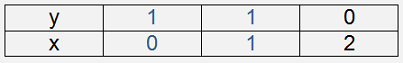
With the two points
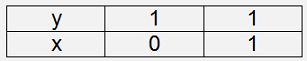
that would be
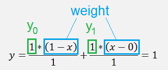
That’s just a straight, horizontal line.
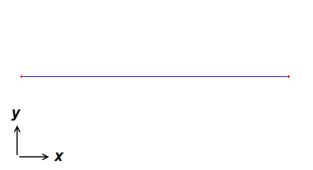
O.k. that’s not too interesting

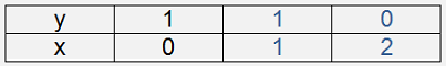
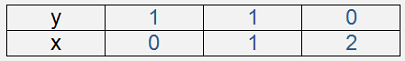
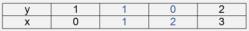
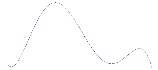
But if we have one additional point like
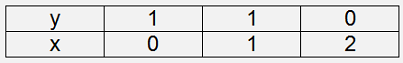
Things become more interesting.
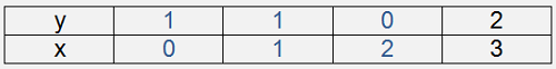
Here, for the 2 points on the left side (blue marked)
we have the same as above
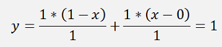
For the 2 points on the right side
we get
That’s the linear equation from the point (1, 1) to (2, 0).
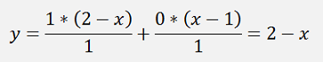
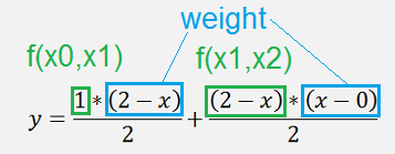
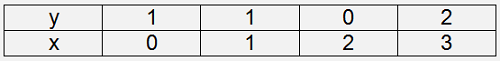
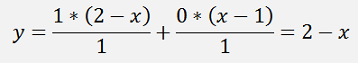
To interpolate over all 3 points
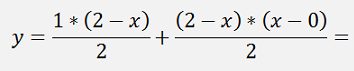
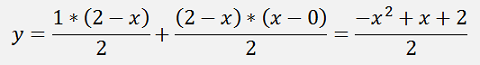
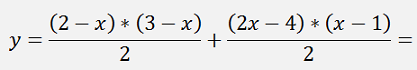
Neville does exactly the same as he did for 2 points. Only that there is no fixed value anymore, but a polynomial function (2 - x) for the 2 points on the right side and, as the interpolation runs over 3 points, we have to divide by 2. Therefore the interpolation polynomial becomes
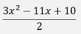
Simplified
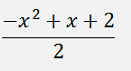
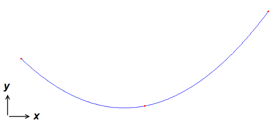
which interpolates the shape
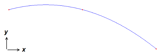
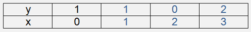
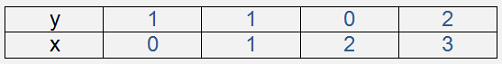
If we get one more point
It’s still the same.
For the 3 points on the left side
It is again the same as above:
For the 3 points on the right side we first have to calculate the interpolations for 2 points:
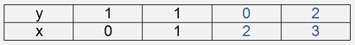
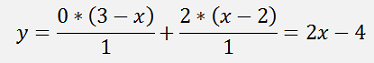
And in the same manner as we did it above, we get the interpolation formula for the 3 points on the right:
That interpolates like:
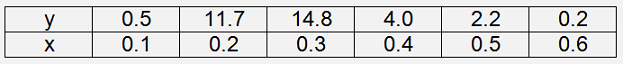
Now we can put these 2 formulas together for all 4 points
and calculate the interpolation polynomial for them. Now we have 2 polynomials of the 2. order, have to divide by 3 and was the polynomial for the 3 points is already a fraction with the value 2 in the denominator, the division is by 6 and the interpolation runs from 0 to 3:
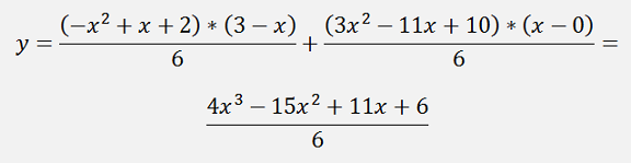
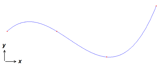
And the final interpolation looks like:
This procedure can be carried out in an iterative loop.
On Wikipedia they show the following table for the generation of the polynomials:
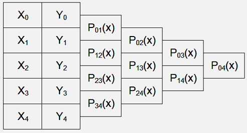
I regard the indexing here as not too useful. But the order is correct. We start at the left side to compute the first row. Then we move to right row by row and run from to bottom to compute each p(x).
For each iteration there is an interpolation range with a starting xs and an ending xe. And there is a polynomial on the left pl(x) and a polynomial on the right side pr(x) coming from the last loop. With this the formula for one new polynomial pn(x) is:
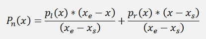
For the first loop the yn values are used as starting polynomials.
Implemented in a small C# function that looks like:
double[] CalcOnePoly(double x_start, double x_end, double[] p_l, double[] p_r, double range)
{
double[] tempP = { -1, x_end};
double[] tempPoly1 = Poly.Mult(p_l, tempP);
tempP[0] = 1;
tempP[1] = -x_start;
double[] tempPoly2 = Poly.Mult(p_r, tempP);
return Poly.Divide(Poly.Add(tempPoly1, tempPoly2), range);
}
With the static class Poly to handle polynomials.
A polynomial is represented in an array of double with the first element the parameter for the x of the highest power.
I use 2 lists
List<double[]> NevillePoly = new List<double[]>();
List<double[]> tempNeville = new List<double[]>();
To carry the polynomials.
The list NevillePoly I initiate with the y values y_k:
for (i = 0; i < order; i++)
{
double[] tempP = { y_k[i] };
NevillePoly.Add(tempP);
}
And compute all the polynomials till only one remains in the list:
void CalcNeville()
{
int i, j;
j = 0;
while(NevillePoly.Count > 1)
{
j++;
tempNeville.Clear();
for (i = 0; i < NevillePoly.Count - 1; i++)
{
double[] tempP1 = NevillePoly[i];
double[] tempP2 = NevillePoly[i + 1];
tempNeville.Add(CalcOnePoly(x_k[i], x_k[i + j], tempP1, tempP2, j));
}
NevillePoly.Clear();
NevillePoly.AddRange(tempNeville);
}
}
At the end there is just one polynomial remaining in NevillePoly. That’s the interpolation polynomial. Quite a simple algorithm
The interpolation for one x is done like:
double Interpolate(double xp)
{
double yp;
double[] p = NevillePoly[0];
int i, k;
yp = 0.0;
for (i = 0; i < p.Length; i++)
{
yp += Math.Pow(xp, p.Length - i - 1) * p[i];
}
return yp;
}
With the same polynomial I already use in the other interpolation algorithms
Neville has no problems and shows:
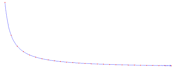
But it tends to oscillate with a bigger number of supporting points. Using y = 1 / x to generate 26 supporting points we get:
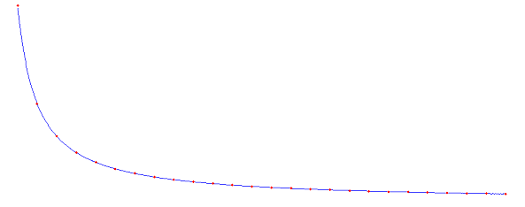
That still looks o.k.
But with the same shape and 28 supporting points the oscillations start at the end of the shape:
At the last 5 points it becomes visible
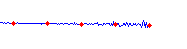
The Neville interpolation algorithm is nice and simple. But it has the same weakness as many other interpolation algorithms. It tends to oscillate with too many supporting points.
To deal with more supporting points I prefer the algorithm introduced by Newton himself (see Newton interpolation). It’s a bit more complicate but it can handle up to 50 supporting points
For other approaches see Polynomial interpolation, Newton interpolation, Newton Gregory interpolation, Interpolation by Chebychev polynomials